Fitting the yield curve

A Work Project, presented as part of the requirements for the Award of a Masters Degree in Finance from the Faculdade de Economia da Universidade de Lisboa.

F

I T T I N G

T

H E

Y

I E L D

C

U R V E

Â

NGELA

G

ERMANO

B

ILHASTRE

126

A Project carried out on the Finance course, with the supervision of:

P

ROFESSOR

P

AULO

L

EIRIA

F

I T T I N G T H E

Y

I E L D

C

U R V E

Abstract

This paper is concerned with the fitting of the yield curve in order to achieve a continuous term structure of interest rates by applying two methods: the cubic polynomial spline by McCulloch (1975), and the Nelson-Siegel-Svensson (1994). Subsequently, a trading model is used to make sensitivity analysis decisions on whether to buy or sell a bond (reach/cheap analysis). Finally, with the purpose of forecasting future yields, out-of-sample forecasts are calculated for the parameters of the Nelson-Siegel-Svensson.

Keywords: Fitting, Yield Curve, McCulloch, Nelson-Siegel-Svensson.

1. Introduction

Interest rates are extremely important for a wide variety of reasons. Either for issuers, dealers, hedgers, investors, or portfolio managers, there is a need to discount future cash-flows, either to price a bond or a derivative product, to construct forward interest rates, or to determine risk premia associated with different maturities (Bolder and Gusba, 2002 and Bolder and Stréliski, 1999).

However, the market term structure of interest rates is discrete and the maturity range available may not be the one we need for valuation purposes, since cash flows do not occur exactly at the times for which market data exists. The term structure can be represented by the spot curve by the discount function or by the forward curve. As long as one of these functions is known, all the other rates can be calculated from the known one (Kappi, 1998).

Therefore, the practical purpose of this paper is to fit the term structure in order to obtain a continuous curve. The interpolation methods used are the cubic polynomial spline-based method, pioneered by McCulloch (1975), and the Nelson-Siegel-Svensson (1994) model, in a maturity range up to 10 years.

The selection of which method to use in practical terms depends on a trade-off between accuracy and ease of computation and on the user’s requirements and planned applications, concerning accuracy, flexibility, consistency, and simplicity of the model (Choudhry, 2005).

Regarding the two methods used in this paper, there are pros and cons in both. The advantages of the cubic polynomial spline-based method are its flexibility and easy usage (Kappi, 1998). However, this method can be too sensitive to changes in parameters, implying rates to fluctuate excessively (Choudhry, 2005), and it might provide unstable estimates of forward rates, especially at longer maturities (Shea, 1984).

The Nelson-Siegel (1987) method is considered to be easier to compute, but not as flexible as the spline-based method, since it only has four parameters and one function for the entire term structure, being able to produce term structures with one hump but not ‘spoon-shaped’ curves with a hump and a trough (James and Webber, 2000). Nevertheless, the extended Nelson-Siegel-Svensson (1994) method, by using six parameters, is able to generate more than one hump, providing more flexibility and, therefore, a better fit than the Nelson-Siegel (1987) model. Contrary to the spline method, both the Nelson-Siegel (1987) and the Svensson extension (1994) models force the long end of the term structure to a horizontal asymptote, the consol rate, and do not require the choice of knot points1.

As soon as the term structure is fitted, a comparison between the interest rates achieved by each method and the ones observed in the market allow for sensitivity analysis decisions and to whether to buy or sell the respective bond (reach/cheap analysis).

Finally, out-of-sample forecasts are calculated for the parameters of the Nelson-Siegel-Svensson. The concentration on these parameters has to do with their economic meaning and also with the yield curve dependency on them when using the Nelson-Siegel-Svensson model, meaning that forecast these parameters is equivalent to forecast the yield curve (Diebold and Li, 2006).

1

2. Literature Review

In order to derive a continuous term structure of interest rates from the observed market prices, several different methods can be used such as simple linear regression, polynomial, exponential or basis splines, the Nelson-Siegel (1987) and its extensions, the bootstrapping method or cubic splines. This paper uses the cubic polynomial spline by McCulloch (1975) method, and the Nelson-Siegel-Svensson (1994) method to fit the yield curve.

The pioneer of the spline-based methods was McCulloch (1975) by introducing the polynomial splines. McCulloch’s work was extended by Vasicek and Fong (1982) with the use of exponential splines. This extension assured that the forward and spot rates would converge to a fixed limit as maturity increases, solving one of the problems of the McCulloch’s method. Fama and Bliss (1987) constructed the yield curve via estimated forward rates at the observed maturities. Furthermore, Kappi (1998) extended the literature of the term structure estimation with splines by applying a smoothing spline method, which uses the square of the discontinuity jump in the third derivatives at the interior knot points and locates the knot points by the size of the fitting errors.

The Nelson-Siegel (1987) approach is considered to be a simple parsimonious model that is flexible enough to represent the shapes generally associated with yield curves: monotonic, humped and S shaped (Nelson and Siegel, 1987). Diebold and Li (2006) show that the parameters of the Nelson-Siegel (1987) method can be interpreted as factors corresponding to level, slope and curvature and uses the model to forecast the yield curve. However, Bolder and Stréliski (1999) decided to employ the Nelson-Siegel-Svensson (1994) method, considering it a good choice given its ability to capture the behaviour of the forward curve. Moreover, Rezende (2008) introduces a new Nelson-Siegel model of six factors, and compares the interpolation abilities of nonparametric

and parametric term structure models widely used by the main Central Banks of the world.

The results taken from past research show that the parsimonious Nelson-Siegel (1987) model outperforms several competitors in forecasting the term structure of interest rates over a one-year horizon (Diebold and Li, 2006). Rezende (2008) demonstrates the superiority of the smoothing spline model in interpolating the spot and the forward curve, compared with the other models presented, although this model turns out to be unstable in fitting the initial rates of the term structure. He also shows the advantage of the six factors extension model over the more simple models in the Nelson-Siegel class, exhibiting smoothness and flexibility.

3. Fitting the Yield Curve 3.1. Methodology

Methods can be distinguished by being linear or non-linear. A linear curve, the case of the spline-based method, is easier to optimise since it forms a vector space with a set of basis elements, implying that each segment can be represented as a linear combination of basis functions. On the other hand, a non-linear curve, the case of Nelson-Siegel-Svensson (1994), may be trickier to optimise since it does not allow the whole curve to be represented by the sum of the segments, as it does not have a set of basis functions (James and Webber, 2000) and (Choudhry, 2005), and also because the results are sensitive to the estimation procedure chosen, for instance the linear or nonlinear least squares, or the starting values used for the parameters.

The price of a coupon bond is the sum of its discounted cash flows (CF), which are the coupons and the face value. However, throughout this paper the bonds used are zero coupon bonds, which price is just the present value of the face value. It should be

noticed that zero coupon bonds are always priced below their face value, or at a discount, because otherwise investors would not have incentive to buy them. Moreover, there is an error (

ε

) when linking model’s prices to observed prices, due to investors’ considerations, including the liquidity of bonds, which is a function, for instance, of issue size, market-maker support and investor demand, the tax treatment of cash flows, or the bid-ask spread (Choudhry, 2005). Therefore, the observed price of a zero coupon bond maturing at time tj, can be described as:

( )

t_j =CF_jd

( )

t_j +ε

P ₍₁₎

Where d(tj) is the discount function, at tj, which is related to the yield y(tj) by the

subsequent equation: 1 ) ( 1 ) ( 1 −         = j j j t d t y (2)

The following section explains the two methods applied in this paper: the cubic polynomial spline, pioneered by McCulloch (1975), and the Nelson-Siegel-Svensson (1994).

3.1.1. The cubic spline-based method by McCulloch (1975)

The spline approach is a linear interpolation technique which splits the term structure of interest rates into segments. The cubic polynomial spline-based method involves a set of functions that define each segment to have third-order polynomials, divided by points, called knots. This degree of spline is the commonly used one, given the fact that it is easy to compute and it does not oscillates much comparing to higher order degree splines (Kappi, 1998).

( )

j i s i i j g t t d

∑

= + = 1 1 ) ( α ₍₃₎

Where g₁

( ) ( )

t_j ,g₂ t_j ,...,g_s

( )

t_j are the set of s basis piecewise cubic functions and

s

α α

α₁, ₂,..., are the unknown parameters that need to be estimated.

McCulloch (1975) makes recommendations for the number of knot points, Ti, that

should be used and for the number of basis functions, s, and, therefore, for the number of segments, (s-2), by which the term structure should be divided. These recommendations were followed throughout this paper. Regarding the position of the knot points, McCulloch (1975) recommends them to be equally divided within each segment, and the use of the following formula, given that the bonds are ordered in ascendant way of maturity

(

t₁ ≤t₂ ≤...≤t_K

)

:

(

)

     − = − ≤ ≤ − + = = ₊ 1 2 2 * 1 0 1 s i t s i t t t i T k h h h i θ (4) Where,     − − = 2 * ) 1 ( s K i INT h , h s K i ₋ − − = 2 * ) 1 (

θ and K is the number of bonds.

Concerning the number of basis functions, McCulloch (1975) suggests that it should be defined as the integer given by the squared root of the number of bonds (K). The value of each basis function is computed by the subsequent formula:

t t g s i Case T t T t T T T T T T t T T T T t T t T t T T T T T t T T T T t T t t g s i Case i i i i i i i i i i i i i i i i i i i i i i i i i i = =            ≥       − + − − − < ≤ − − − − + − − + − < ≤ − − < = < + + − + − + + + − − − − − − ) ( : 2 2 6 * 2 * ) ( ) ( * 6 ) ( 2 ) ( 2 ) ( * ) ( 6 ) ( ) ( * 6 ) ( 0 ) ( : 1 1 1 1 1 1 1 1 1 3 2 1 2 1 1 1 3 1 1 (5)

From the Equation (3) of the discount function, the price of a zero coupon bond maturing at date tj can be rewritten as:

( )

_∑

( )

= = − s i j i j i j j CF CF g t t P 1 α ₍₆₎

The unknown parameters

α

_i were estimated with an ordinary least squares (OLS) regression, which is possible since the spline-based method produces a continuous and linear function (Choudhry, 2005). Having the parameters, the discount function can be calculated from Equation (3) and, consequently, the prices and zero coupon yields respectively from Equations (1) and (2).

3.1.2. The Nelson-Siegel-Svensson (1994)

The Nelson-Siegel (1987) method uses a single exponential function for the entire term structure, with four parameters. Although in most cases this original model gives a reasonable fit, for more complex shapes of the yield curve it is unsatisfactory. Consequently, in order to circumvent the lack of flexibility of the original model, some extensions have been made.

The Nelson-Siegel-Svensson (1994) is one of these extensions, adding one exponential component to the original model. The structure of this extension for the yield, y(tj), with six estimated parameters, α1,α2,α3,α4,β1,and

β

2, is given by:

( )

        −         − +         −         − +         − + = ₁ − 1 ₁ − 1 − 1 2 ₁ − 2 − 2 4 1 3 1 2 1 β β β β β _α β _α β β α α j j j j j t t j t t j t j j e e t e e t e t t y ₍₇₎

One of the advantages of the Nelson-Siegel-Svensson (1994) is that the estimated parameters have economic meaning. This can easily be seen if

β

₁ and

β

₂ are fixed and the derivative of the yield is taken relative to each of the remaining parameters

α

₁,

α

₂,

3

α and

α

₄. In this case,

α

₁ is interpreted as the short term rate in the long term, or the consol rate, and it represents parallel changes of the term structure;

α

₂ is the slope of the term structure or, in other words, the spread between the consol rate and the instantaneous short rate, where the instantaneous short rate is the sum of

α

₁and

α

₂; and, finally, α₃ and

α

₄ are associated to the first and second curvatures of the term structure, so that negative values of these variables imply convex shapes, and positive values lead to concave shapes. Concerning the parameters

β

₁ and

β

₂, they are related to the speed of convergence of the term structure towards the consol rate

α

₁, with higher values of these variables being associated with a lower speed, and vice-versa.

The appropriate value for the betas can be achieved by trial and error, implying the setting of provisional values, and the computation of many regressions, in order to obtain the overall best fitting values for the parameters, which are the ones that generate lower errors. However, rather little precision of fit is lost if a median value is imposed for all data sets (Nelson and Siegel, 1987). Having this in mind, the betas were fixed at values that minimize the sum of squared errors, in which the errors are the difference

between observed yields and the yields obtained by the model, subject to the constraint that the betas are positive, and the alphas were estimated using an OLS regression. The OLS method is simpler and it also enhances numerical trustworthiness by enabling us to replace hundreds of potentially challenging numerical optimizations (Diebold and Li, 2006).

However, volatility of prices is not the same across the maturity spectrum, for instance short term yields are more volatile than long term yields. Therefore, each yield error should be weighted by a value related to the inverse of its duration (Bolder and Stréliski, 1999), being the duration a measure of sensitivity of the bond price to changes in interest rates. Consequently, the minimization problem is the following:

0 0 . . 1 1 2 1 2 , 2 1 > ∧ >                           ×

∑ ∑

∑

= = β β ε β β t s D D Min c a m n j m n j j j (8)

Where a and c are the sample period, n and m are the interval of the maturities of the bonds, and D is the Macaulay duration (_j D_mac) of the jth bond. The Macaulay duration is a weighted average maturity of a bond and it provides an understanding of the relationship between interest rates and prices, implying that for a given change in interest rates the change in price will be greater for a longer-term bond than for a shorter-term bond (Bolder and Stréliski, 1999). The duration of a zero coupon bond, the ones that are being used in this paper, is equal to its time to maturity, implying the duration weights to be fixed throughout the sample used.

3.2. Data

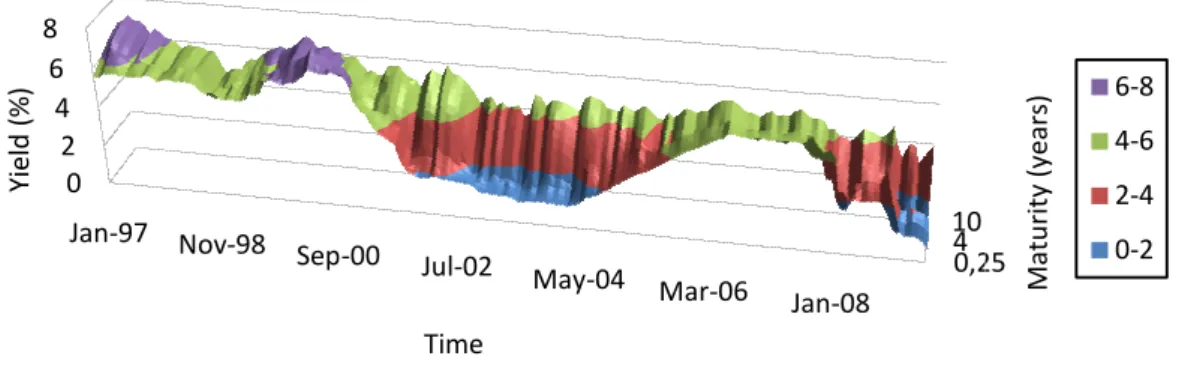
The data set used in this paper includes United States of America (U.S.) and Germany zero coupon yields, with maturities ranging from 3 months to 10 years, obtained from Reuters. The sample contains, respectively for U.S. and Germany, 149 and 137 monthly observations related to the last day of each month in the period from January 1997 for U.S., and January 1998 for Germany, to May 2009. Figure 1 (a) and (b) show a three-dimensional plot of historical yield curves where the large amount of temporal variability is evident, either in level or in slope. Table 1 (a) and (b) provide descriptive statistics for monthly yields at different maturities, and for the yield curve level, slope and curvature, using the definition of Diebold and Li for these terms. The level of the yield curve is therefore defined as the yield at the highest maturity, which in this case is ten years, the slope is the difference between the ten and the three month yield to maturity, and the curvature is twice the two year yield minus the sum of the three month and ten year yields to maturity. From Table 1 it is possible to state that the typical yield curve is upward sloping and that volatility decreases with maturity. Moreover, the level appears to change moderately relative to its mean, while slope and curvature change significantly comparative to their mean. Figure 2 shows once again the upward sloping trend of yield curves and also illustrate that short term yields are more volatile than long term yields. Moreover, U.S. yields were higher than Germany yields during the first years of the sample, and since then remain similar. Figure 3 (a) also highlights the fact that U.S. yields were higher at the beginning of the sample years but had a decreasing trend throughout the first years of the sample, remaining fairly stable from then on. Moreover, the slope, illustrated by the long rate premium, appears to change significantly during the sample period leading to varying shapes of the yield curve at each specific time. On the other hand, Figure 3 (b) shows that Germany yields

remained quite stable in level during the sample period. Concerning the relationship between long and short yields, inverted yield curves were only common at the end of the sample period.

3.3. Estimation Procedure

In order to verify the ability of both models to fit different shapes of the yield curve, three moments in time were selected from the sample of each country, namely moments that exhibited positively sloped, flat and inverted shapes. The two models are applied in the U.S. on January 1998, December 2000 and March 2002 and in Germany on December 2000, May 2004 and March 2008. Moreover, the descriptive statistics of the estimated factors, the average performance of both models against the average market data and the residuals are also illustrated.

3.3.1. The cubic spline-based method by McCulloch (1975)

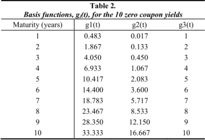
Since the McCulloch suggestions were taken into account, and our sample contains 10 zero coupon yields2 at each point in time, there are three basis functions, s. Therefore, the number of segments is 1 and the number of knot points is 2, placed at 0 and 10 years to maturity as stated by Equation (4). Table 2 presents the results of the basis functions, implied by Equation (5). Then, the product between the basis functions and a matrix of cash flows of the zero coupon bonds3 is the independent variable in the OLS estimation, as defined on the right side of Equation (6). The dependent variable is the price observed in the market at each point in time minus 100 which is the cash flow of a zero coupon bond. The descriptive statistics of the alphas of Equation (6), obtained

2

The McCulloch method does not take into account the differences in volatility implying the results for the money market to be inaccurate. In order to overcome this problem it was decided to work on this model only with the bond market, therefore from one year to ten year to maturity zero coupon yields. 3

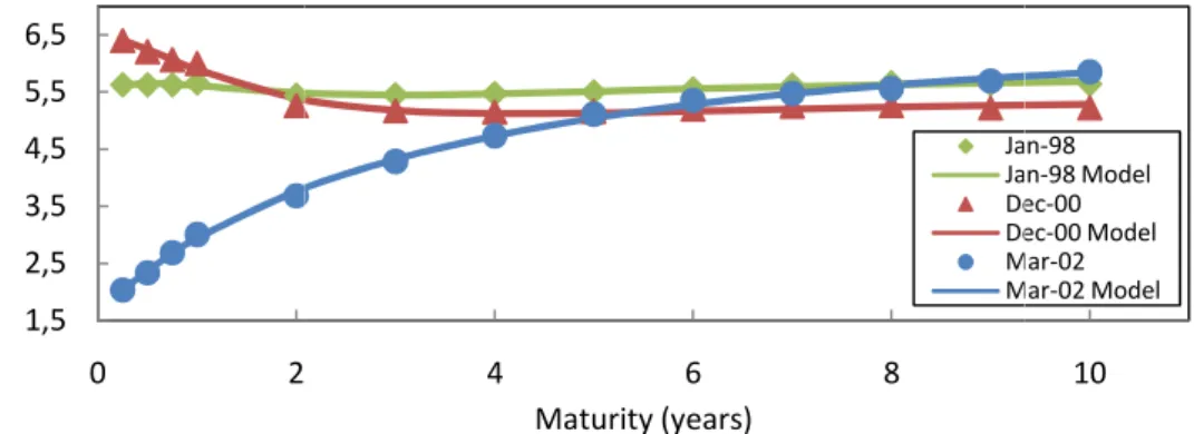
from the OLS regression, are presented in Table 3. The mean alphas are very similar for both countries, having -0.0021, 0.0025 and -0.0356, respectively, for alpha 1, alpha 2 and alpha 3 for U.S., and -0.0026, 0.0026 and -0.0302, respectively, for Germany alpha 1, alpha 2 and alpha 3. However, U.S. alphas change more relative to their mean than Germany alphas. The discount function is then calculated by Equation (3), and therefore the model zero coupon yields and the model prices can be found. In Figure 4, the estimated average fitted yield curve is plotted against the average market yield curve and Figure 5 (a) and (b) illustrates the results for the model zero coupon yields at the three selected dates. Regardless the country or the shape of the yield curve, the highest maturities were effectively fitted. However, although the McCulloch model is said to be more flexible, its performance to what concerns the lower maturities of the yields was not as good as expected. Despite this fact, the errors, which are the differences between the market yields and the estimated model yields, are quite small during the entire sample period, ranging from -0.7% to 2.3% for U.S. and from -0.3% to 2.1% for Germany, as illustrated in Figure 6 (a) and (b).

3.3.2. The Nelson-Siegel-Svensson (1994)

As stated before, the approach of the Nelson-Siegel-Svensson method taken in this paper considers that β1 and β2 _{are fixed at median values that minimise the sum of}

squared errors. The estimated betas for U.S. are 0.5803 and 1.3131, respectively, for β1

and β2, and 0.5897 and 1.4413 for Germany.

Once the betas are fixed, the factor loadings of the model, illustrated in Figure 7, can be computed, being these the independent variables in the OLS regression. The loading of alpha 1 is constant at 1, representing the level factor. The loading of alpha 2

is _       − − 1 1 1 β β tj j e

t , a function that starts at 1 and decays quickly to 0, representing the slope factor. And, finally, the loadings of alpha 3 and alpha 4 are, respectively,

1 1 1 1 β β β tj tj j e e t − − −         − and β2 ₁ β2 β2 j j t t j e e t − − −        

− , both functions that start at zero, increase,

and then decay to zero again, representing the first and second curvatures of the term structure. The dependent variables in the OLS regression are the zero coupon yields observed in the market. Table 4 presents the descriptive statistics of the OLS estimated parameters. For the U.S., the estimated alphas indicate that the short term rate in the long term is around 5.76% on average, when the actual average for level is 5.02%. The average alpha 2 is negative implying an average positive slope, just like the sign of the actual mean slope. Finally, since the estimated alpha 3 and alpha 4 are negative, the first curvature has a concave shape on average because the loading of alpha 3 is negative, and the second curvature has a convex shape on average because the loading on alpha 4 is positive. For Germany, the average estimated consol rate is 5.06%, which compares with 4.36% for the actual mean of the sample period. The estimations indicate, for Germany, again a positive slope on average, a concave shape for the first curvature and a convex shape for the second curvature, on average, in the term structure. Having the estimated alphas, the zero coupon yields of the model can then be determined by Equation (7) and are represented in Figure 8 as an average against the average market yield curve, and also in Figure 9 (a) and (b) for the three selected dates. The model performance, both for the U.S. and Germany, appears to be very good for all maturities, presenting errors ranging from 0.4% and -0.7%, as illustrated in Figure 10 (a) and (b).

3.4. Trading Model

As soon as the term structure is fitted, a comparison between the prices achieved by each method and the ones observed in the market allow for sensitivity analysis decisions. Therefore, when the market prices are above the model prices the bond is thought to be overpriced and the advisable action is to sell the bond. On the other hand, when the market price is below the model price, the bond is believed to be underpriced and the advisable action is to buy it. Figure 11 (a) and (b) illustrates the trading model for two different advisable actions for both models.

3.5. Nelson-Siegel-Svensson parameters behaviour and forecasting

As explained before, the parameters of the Nelson-Siegel-Svensson model have economic meaning making worthwhile to study their behaviour throughout time and also to forecast them. This is confirmed by Figure 12 where the parameters of the model are plotted along with the empirical level, slope and curvature. The correlation coefficients, respectively for U.S. and Germany, for alpha 1 and level are 68% and 80%, for alpha 2 and slope are 94% and 93%, for alpha 3 and curvature 36% and 27%, and, finally, for alpha 4 and curvature 92% and 95%.

In order to forecast α1t α2t α3t and α4t, the full data sample was divided into initial

estimation period and forecasting period (De Pooter, 2007). Therefore, the estimation period for the U.S. goes from January 1997 to March 2003 (75 observations), and the forecasting period goes from April 2003 to May 2009 (74 observations), and for Germany it goes, respectively, from January 1998 to September 2003 (69 observations), and from October 2003 to May 2009 (68 observations). The purpose of this division is to use out-of-sample criteria, which is better for forecasting as it allows the evaluation

of the forecasts capabilities of the model (Wooldridge, 2002). The forecast of the alpha αi(b+1) is: ib i i b i δ δ α α₍ +₁₎ = ₀ + ₁* (9)

Where δi0 and δi1 are estimated by OLS for 1-month, 3-month and 6-month-ahead,

and b is the alpha value in the month before the forecast. The results for the forecasted alphas are quite good with correlations always higher than 70% between the forecasted variables and the estimated ones, shown in Table 8.

Having the forecasted alphas, it is possible to forecast the yield curve using the Nelson-Siegel-Svensson model equation, as the yield curve depends only on these parameters (Diebold and Li, 2006). The forecasted yield, y(tj)(b+1), is therefore described

by the following equation:

        −         − +         −         − +         − + = + − − − − + − + + + 1 1 1 1 1 1 2 2 ) ( 2 ) 1 ( 4 1 ) 1 ( 3 1 ) 1 ( 2 ) 1 ( 1 ) 1 ( β β β β β _α β _α β β α α j j j j j t t j b t t j b t j b b b j e e t e e t e t t y ₍₁₀₎

The forecast error, which is only known at b+1, is the difference between the actual occurred yield and the forecasted value:

) 1 ( ) 1 ( ( ) ( ) ) (t_{j b+} = y t_{j actual}− y t_{j b+} e ₍₁₁₎

The forecasted errors, shown in Tables 6, 7 and 8, are between 1% and -1% on average indicating a good performance of the forecasts. For the three steps-ahead forecasts studied and almost all maturities, the mean forecasted errors are smaller for U.S., although they change more, than they are for Germany. The higher mean forecasted errors happen at 1-year and 2-year maturities, for both countries and for the three steps-ahead forecasts. As expected, the root mean squared error (RMSE), defined as the root of the squared errors averaged over the sample, increase with higher steps ahead in time.

4. Conclusion

Given the huge importance of interest rates, this paper explores the fitting of the yield curve by two models: the cubic spline-based method by McCulloch (1975) and the Nelson-Siegel-Svensson (1994). The results show that the Nelson-Siegel-Svensson model provides smaller errors for fitting the yield curve when compared with the McCulloch model, although the opposite was expected given the higher flexibility of the latter. Moreover, the Nelson-Siegel-Svensson allows for the introduction of duration weights, accounting for different volatilities in yields, and its parameters have economic meaning.

A simple and user-friendly trading model is also developed based on the results of both methods. It should not be forgotten that the differences between the market data and the model estimations could be explained by investors’ considerations, including the liquidity of bonds, which is a function, for instance, of issue size, market-maker support and investor demand, the tax treatment of cash flows, or the bid-ask spread.

The economic meaning of Nelson-Siegel-Svensson parameters explains the concern of this paper on their behaviour and forecast. The results demonstrate high correlations between the parameters and the empirical values of level, slope and curvature of yields. Furthermore, the forecasting results appear to be very efficient, with high correlations between the parameters and the forecasts, and also small forecast yield errors.

5. References

Adams, K.J. and Donald R. Van Deventer. 1994. “Fitting the Yield Curves and Forward Rate Curves with Maximum Smoothness”. Journal of Fixed Income, 4(1): 52-62. Bolder, D.J. and David Stréliski. 1999. “Yield Curve Modelling at Bank of Canada”.

Bank of Canada, Technical Report No. 84.

Bolder, D.J. and Scott Gusba. 2002. “Exponentials, Polynomials, and Fourier Series: More Yield Curve Modelling at the Bank of Canada”. Bank of Canada, Working Paper 2002-29.

Choudhry, Moorad. 2005. “Fitting the Yield Curve” In Fixed-Income Securities and Derivatives Handbook – Analysis and Valuation, 1st edition, 83-92. Princeton: Bloomberg Press.

De Pooter, Michiel. 2007. “Examining the Nelson-Siegel Class of Term Structure Models: In-sample fit versus out-of-sample forecasting performance”. Econometric Institute and Tinbergen Institute, Erasmus University Rotterdam, Netherlands.

Diebold, Francis X. and Canlin Li. 2006. “Forecasting the Term Structure of Government Bond Yields”. Journal of Econometrics, 130: 337-364.

Fama, F. and Robert R. Bliss. 1987. “The Information in Long-Maturity Forward Rates”. American Economic Review, 37(4): 680-692.

Hull, John C. 2006. “Interest Rate Derivatives: Models of the Short Rate” In Options, Futures and Other Derivatives, 6th edition, 649-674. New Jersey: Prentice Hall. Hunt, Benjamin Francis. 1995. “Fitting Parsimonious Yield Curve Models to Australian

Coupon Bond Data”. School of Finance and Economics, University of Technology Sydney, Working Paper no. 51.

James, Jessica and Nick Webber. 2000. “Modelling the Yield Curve” In Interest Rate Modelling: Financial Engineering, 425-453. Wiley.

Kappi, Jari. 1998. “Estimating a Smooth Term Structure of Interest Rates”, Helsinki School of Economics and Business Administration, 159-177.

McCulloch, J. Huston. 1975. “The Tax-Adjusted Yield Curve” In Journal of Finance, 30(3): 811-830.

Nelson, Charles R. and Andrew F. Siegel. 1987. “The Parsimonious Modeling of Yield Curves” In Journal of Business, 60(4): 473-489.

Rezende, Rafael B. 2008. “Giving Flexibility to the Nelson-Siegel Class of Term Structure Models”, Center for Development and Regional Planning. Brazil.

Shea, Gary S. 1985. “Interest Rate Term Structure Estimation with Exponential Splines: A Note” In Journal of Finance, 40(1): 319-325.

Svensson, L. E. 1994. “Estimating and Interpreting Forward Interest Rates: Sweden 1992-1994”, International Monetary Fund, Working Paper No. 114.

Vasicek, Oldrich A. and H. Gifford Fong. 1982. “Term Structure Modeling Using Exponential Splines” In Journal of Finance, 37(2): 339-348.

Wooldridge, Jeffrey M. 2002. “Advanced Time Series Topics” In Introductory Econometrics: A Modern Approach, 571-615. 2 E South Western College.

Figure 1 (a). Historical U.S. yields.

Figure 1 (b). Historical Germany

Descriptive statistics for U.S

Maturity (years) Mean Std. Dev. 0.25 3.942 1.874 0.5 4.035 1.838 0.75 4.104 1.818 1 4.186 1.793 2 3.948 1.719 3 4.145 1.546 4 4.321 1.402 5 4.477 1.292 6 4.621 1.193 7 4.755 1.096 8 4.861 1.004 9 4.936 0.919 10 (Level) 5.018 0.853 Slope 1.076 1.423 Curvature -1.063 1.115 Number of observations = 149 Jan-97 _Nov-98 Sep 0 2 4 6 8 Y ie ld ( % )

Jan-98 Jul-99 _Jan-01

0 2 4 6 Y ie ld ( % ) 6. Appendices yields.

istorical Germany yields.

Table 1.

Descriptive statistics for U.S. and Germany zero coupon yields

U.S Germany

(%) (%)

Std. Dev. Min Max Mean Std. Dev.

1.874 0.674 6.863 3.310 1.000 1.270 1.838 1.119 7.105 3.367 1.001 1.471 1.818 1.140 7.333 3.418 1.003 1.568 1.793 1.190 7.501 3.475 1.007 1.638 1.719 0.630 6.910 3.399 0.900 1.320 1.546 0.950 6.760 3.586 0.836 1.700 1.402 1.160 6.830 3.745 0.782 2.020 1.292 1.310 6.900 3.875 0.737 2.290 1.193 1.640 6.970 4.006 0.703 2.520 1.096 2.160 7.040 4.141 0.683 2.720 1.004 2.540 7.090 4.249 0.661 2.900 0.919 2.790 7.100 4.307 0.626 3.070 0.853 2.990 7.110 4.358 0.594 3.170 1.423 -1.179 3.820 1.048 0.865 -1.115 -4.626 0.780 -0.869 0.743

-Number of observations = 149 Number of observations = 137

Sep-00 _Jul-02 May-04 _Mar-06 Jan-08 0,25 4 10 Time 01 _Jul-02 Jan-04 _Jul-05 Jan-07 _Jul-08 0,25 4 10 Time Germany Min Max 1.270 5.277 1.471 5.377 1.568 5.415 1.638 5.495 1.320 5.260 1.700 5.280 2.020 5.290 2.290 5.320 2.520 5.400 2.720 5.530 2.900 5.600 3.070 5.600 3.170 5.600 -1.127 2.680 -3.620 0.549 Number of observations = 137 0,25 M a tu ri ty ( y e a rs ) 6-8 4-6 2-4 0-2 0,25 Ma tu ri ty ( y e a rs ) 4-6 2-4 0-2

0 1 2 3 4 5 6 7 8

Jan-97 Oct-99 Jul-02 Apr-05 Jan-08

Y ie ld ( % ) Time 0.25 YTM 2 YTM 10 YTM 0 1 2 3 4 5 6

Sep-97 Jun-00 Mar-03 Dec-05 Sep-08

Y ie ld ( % ) Time 0.25 YTM 2 YTM 10 YTM

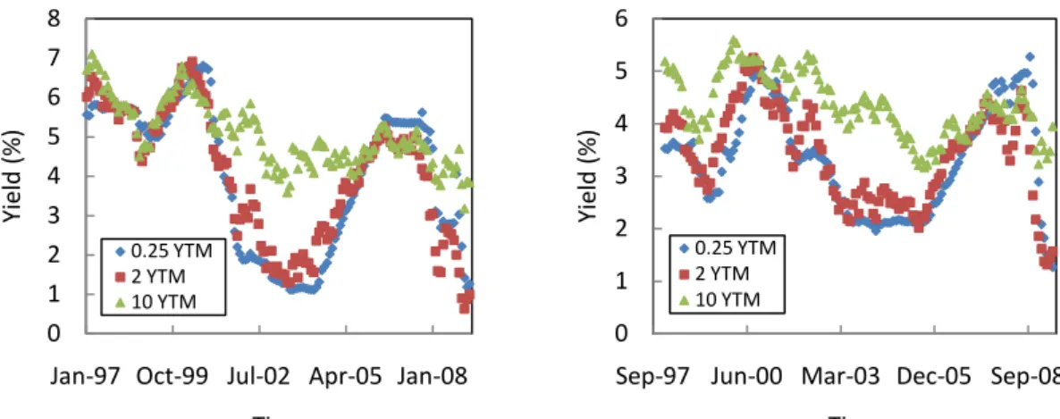
Figure 2. Time series of U.S. (on the left) and Germany (on the right) yields. The yields shown have three-month, two-year, and ten-year maturities (YTM).

Figure 3 (a). Interest rate dynamics of U.S. yields.

Figure 3 (b). Interest rate dynamics of Germany yields.

-2 -1 0 1 2 3 4 5 0 2 4 6 8

Jan-97 Jun-98 Nov-99 Apr-01 Sep-02 Feb-04 Jul-05 Jan-07 Jun-08

Lo n g r a te p re m iu m ( % ) Y ie ld l e v e l (% ) Time Slope Level -2 -1 0 1 2 3 0 1 2 3 4 5 6

Jan-98 Mar-99 May-00 Jul-01 Sep-02 Nov-03 Jan-05 Mar-06 May-07 Lo

n g r a te p re m iu m ( % ) Y ie ld l e v e l (% ) Time Slope Level

3,6 4,1 4,6 5,1 0 5 10 Y ie ld ( % ) Maturity (years) 3 3,5 4 4,5 0 5 10 Y ie ld ( % ) Maturity (years) Table 2.

Basis functions, gi(t), for the 10 zero coupon yields

Maturity (years) g1(t) g2(t) g3(t) 1 0.483 0.017 1 2 1.867 0.133 2 3 4.050 0.450 3 4 6.933 1.067 4 5 10.417 2.083 5 6 14.400 3.600 6 7 18.783 5.717 7 8 23.467 8.533 8 9 28.350 12.150 9 10 33.333 16.667 10 Table 3.

Descriptive statistics of the parameters of the McCulloch method for U.S. and Germany

U.S. Germany

(%) (%)

Mean Std. Dev. Min Max Mean Std. Dev. Min Max

Alpha 1 -0.0021 0.0054 -0.0138 0.0055 -0.0026 0.0032 -0.0086 0.0039

Alpha 2 0.0025 0.0029 -0.0054 0.0092 0.0026 0.0023 -0.0033 0.0079

Alpha 3 -0.0356 0.0194 -0.0677 0.0007 -0.0302 0.0103 -0.0500 -0.0087

Number of obsevations =149 Number of observations = 137

Figure 4. Market (points in graphs) and McCulloch model average yield curve (line in graphs) for U.S.

Figure 5 (a). Market and McCulloch model yield c

March 2002.

Figure 5 (b). Market and McCulloch model yield c

March 2008.

Figure 6 (a). Yield curve Residuals

Figure 6 (b). Yield curve Residuals 2,5 3,5 4,5 5,5 6,5 0 2 Y ie ld ( % ) 2 2,5 3 3,5 4 4,5 5 0 2 Y ie ld ( % ) -1 0 1 2 Jan-97 Dec-98 E rr o rs ( % ) -1 0 1 2 Jan-98 Dec-E rr o rs ( % )

lloch model yield curves for U.S. at January 1998, December 2000 and

). Market and McCulloch model yield curves for Germany at December 2000, May 2004 and

Residuals of the McCulloch method for U.S..

urve Residuals of the McCulloch method for Germany.

4 6 8 Maturity (years) Jan Jan Dec Dec Mar Mar 4 6 8 Maturity (years) Dec Dec May May Mar Mar 17 98 Nov-00 _Oct-02 Sep-04 _Aug-06 M a tu ri ty ( y e a rs ) Time 17

-99 Nov-01 Oct-03 _Sep-05

Aug-07 M a tu ri ty ( y e a rs ) Time

U.S. at January 1998, December 2000 and

cember 2000, May 2004 and 10 Jan-98 Jan-98 Model Dec-00 Dec-00 Model Mar-02 Mar-02 Model 10 Dec-00 Dec-00 Model May-04 May-04 Model Mar-08 Mar-08 Model M a tu ri ty ( y e a rs ) _2-3 1-2 0-1 -1-0 M a tu ri ty ( y e a rs ) _2-3 1-2 0-1 -1-0

-0,4 -0,2 0 0,2 0,4 0,6 0,8 1 0 2 4 6 8 10 (% ) Maturity (years) Level Slope Curvature 1 Curvature 2 -0,4 -0,2 0 0,2 0,4 0,6 0,8 1 0 5 10 (% ) Maturity (years) Level Slope Curvature 1 Curvature 2 3,2 3,4 3,6 3,8 4 4,2 4,4 4,6 0 5 10 Y ie ld ( % ) Maturity (years)

Figure 7. Nelson-Siegel-Svensson loadings for U.S. (on the left) and for Germany (on the right). The β1 and β2 are fixed, respectively, at 0.5803 and 1.3131 for U.S., and at 0.5897 and 1.4413 for Germany.

Table 4.

Descriptive statistics of the parameters of the Nelson-Siegel-Svensson method for U.S. and Germany

U.S. Germany

(%) (%)

Mean Std. Dev. Min Max Mean Std. Dev. Min Max

Alpha 1 5.7606 0.6404 4.3555 7.5582 5.0583 0.6045 3.6499 6.1696

Alpha 2 -2.0969 1.9675 -6.5012 0.9643 -1.8808 1.0122 -4.5537 -0.1170

Alpha 3 -2.1813 3.0634 -15.2270 3.4489 -0.7119 2.0956 -9.1071 2.2892

Alpha 4 -5.6081 4.8854 -25.2264 0.1031 -4.2295 2.6587 -15.3111 -0.3841

Number of observations = 149 Number of observations = 137

Figure 8. Market (points in graphs) and Nelson-Siegel-Svensson model average yield curve (lines in graphs) for U.S. (on the left) and for Germany (on the right).

3,8 4 4,2 4,4 4,6 4,8 5 5,2 0 5 10 Y ie ld ( % ) Maturity (years)

Figure 9 (a). Market and Nelson-2000 and March 2002.

Figure 9 (b). Market and Nelson May 2004 and March 2008.

Figure 10 (a). Yield curve Residuals

Figure 10 (b). Yield curve Residuals 1,5 2,5 3,5 4,5 5,5 6,5 0 2 Y ie ld ( % ) 1,5 2,5 3,5 4,5 5,5 0 2 Y ie ld ( % ) -1 -0,5 0 0,5 Jan-97 Feb E rr o rs ( % ) -1 -0,5 0 0,5 Jan-98 Dec E rr o rs ( % )

-Siegel-Svensson model yield curves for U.S. at January 1998, December

ket and Nelson-Siegel-Svensson model yield curves for Germany

urve Residuals of Nelson-Siegel-Svensson for U.S..

urve Residuals of Nelson-Siegel-Svensson for Germany.

4 6 8 Maturity (years) Jan Jan Dec Dec Mar Mar 2 4 6 8 Maturity (years) Dec Dec May May Mar Mar 0.254 10 Feb-99 Mar-01

Apr-03 May-05 _Jun-07

Time

0.254 10

Dec-99 Nov-01 _Oct-03

Sep-05 _Aug-07

Time

U.S. at January 1998, December

at December 2000, 10 Jan-98 Jan-98 Model Dec-00 Dec-00 Model Mar-02 Mar-02 Model 10 Dec-00 Dec-00 Model May-04 May-04 Model Mar-08 Mar-08 Model M a tu ri ty ( y e a rs ) 0-0,5 -0,5-0 -1--0,5 0.25 10 M a tu ri ty ( y e a rs ) _0-0,5 -0,5-0 -1--0,5

64,0 64,2 64,4 64,6 64,8 65,0 65,2 65,4 65,6 65,8 66,0 7,9 7,95 8 P ri ce Maturity (years) Mar Mar SELL 87,0 87,2 87,4 87,6 87,8 88,0 3,9 3,95 4 P ri ce Maturity (years) May May BUY

Figure 11 (a). Trading Model. The market point at the graph on the left is for McCulloch model

Figure 11 (b). Trading Model. The market point in both graphs is for Germany price line at the graph on the left is for Mc

73 73,1 73,2 73,3 73,4 73,5 73,6 73,7 5,95 6 P ri ce Maturity (years) Mar Mar BUY 8,05 8,1 Maturity (years) Mar-02 Mar-02 Model 4,05 4,1 Maturity (years) May-04 May-04 Model 79 79,1 79,2 79,3 79,4 79,5 79,6 79,7 79,8 79,9 80 5,9 5,95 6 P ri ce Maturity (years) SELL

The market point in both graphs is for U.S. price at March is for McCulloch model and on the right for the Nelson-Siegel-Svensson

The market point in both graphs is for Germany price graph on the left is for McCulloch model on the right for the

Nelson-Siegel-6,05 Maturity (years) Mar-02 Mar-02 Model 6,05 6,1 Maturity (years) May-04 May-04 Model

March 2002. The line Svensson.

The market point in both graphs is for Germany price at May 2004. The -Svensson.

3 3,5 4 4,5 5 5,5 6 6,5

Jan-98 Jan-01 Jan-04 Jan-07

(% ) Time Alpha 1 Level -2 -1 0 1 2 3 4 5

Jan-98 Jan-01 Jan-04 Jan-07

(% ) Time Alpha 2 Slope -16 -14 -12 -10 -8 -6 -4 -2 0 2

Jan-98 Jan-01 Jan-04 Jan-07

(% ) Time Alpha 3 Alpha 4 Curvature 3 3,5 4 4,5 5 5,5 6 6,5 7 7,5 8

Jan-97 Mar-00 May-03 Jul-06

(%

)

Time

Alpha 1 Level

Figure 12.1. Model-based level (α1) versus data-based level for U.S. (on the left) and Germany (on the

right). The correlation coefficient between these two variables is 0.6816 and 0.8029, respectively, for each country.

Figure 12.2. Model-based slope (α2) versus data-based slope for U.S. (on the left) and Germany (on the

right). The correlation coefficient between these two variables is 0.9444 and 0.9272, respectively, for each country.

Figure 12.3. Model-based curvature (α3 and α4) versus data-based curvature for U.S. (on the left) and for

Germany (on the right). The correlation coefficient between these variables with curvature is 0.363 and 0.9225, respectively, for α3 and α4 for U.S., and 0.2669 and 0.9472, respectively, for α3 and α4 for Germany. -2 -1 0 1 2 3 4 5 6 7

Jan-97 Mar-00 May-03 Jul-06

(% ) Time Alpha 2 Slope -30 -25 -20 -15 -10 -5 0 5

Jan-97 Mar-00 May-03 Jul-06

(% ) Time Alpha 3 Alpha 4 Curvature

Table 5.

Correlation coefficients between forecasted alphas and actual alphas of Nelson-Siegel-Svensson

U.S. Germany α1 α2 α3 α4 α1 α2 α3 α4 F o re ca st ed h=1 α1 0.7132 - - - 0.8871 - - - α2 - 0.9669 - - - 0.9616 - - α3 - - 0.9475 - - - 0.9515 - α4 - - - 0.9472 - - - 0.9075 h=3 α1 0.7121 - - - 0.8860 - - - α2 - 0.9670 - - - 0.9614 - - α3 - - 0.9498 - - - 0.9498 - α4 - - - 0.9490 - - - 0.9114 h=6 α1 0.7097 - - - 0.8824 - - - α2 - 0.9671 - - - 0.9613 - - α3 - - 0.9502 - - - 0.9493 - α4 - - - 0.9497 - - - 0.9124 Table 6.

Descriptive statistics for 1-month-ahead U.S. and Germany Forecasted Errors

Maturity (years)

U.S. Germany

(%) (%)

Mean Std. Dev. RMSE Mean Std. Dev. RMSE

0.25 -0.0225 0.3239 0.3225 -0.0383 0.2680 0.2688 0.5 -0.0398 0.2954 0.2961 -0.0568 0.2772 0.2809 0.75 -0.0044 0.2780 0.2761 -0.0255 0.2619 0.2612 1 0.0880 0.2627 0.2754 0.0387 0.2471 0.2483 2 -0.1540 0.3420 0.3730 -0.1536 0.3731 0.4009 3 0.0006 0.3210 0.3188 -0.0373 0.2646 0.2369 4 0.0160 0.3148 0.3131 -0.0104 0.2384 0.2310 5 -0.0167 0.3079 0.3063 -0.0206 0.2317 0.2268 6 -0.0468 0.3102 0.3116 -0.0359 0.2256 0.2197 7 -0.0557 0.3067 0.3097 -0.0447 0.2167 0.2137 8 -0.0545 0.3014 0.3043 -0.0492 0.2095 0.2103 9 -0.0500 0.2977 0.2999 -0.0511 0.2055 0.2310 10 -0.0282 0.2998 0.2991 -0.0437 0.2031 0.2063

Table 7.

Descriptive statistics for 3-month-ahead U.S. and Germany Forecasted Errors

Maturity (years)

U.S. Germany

(%) (%)

Mean Std. Dev. RMSE Mean Std. Dev. RMSE

0.25 -0.0254 0.3245 0.3233 -0.0402 0.2784 0.2792 0.5 -0.0424 0.2957 0.2968 -0.0587 0.2917 0.2954 0.75 -0.0073 0.2792 0.2775 -0.0279 0.2794 0.2788 1 0.0846 0.2634 0.2750 0.0356 0.2661 0.2665 2 -0.1596 0.3490 0.3816 -0.1590 0.3885 0.4171 3 -0.0059 0.3237 0.3216 -0.0436 0.2776 0.2790 4 0.0096 0.3188 0.3168 -0.0169 0.2491 0.2479 5 -0.0227 0.3148 0.3135 -0.0269 0.2423 0.2420 6 -0.0523 0.3178 0.3200 -0.0417 0.2368 0.2387 7 -0.0607 0.3134 0.3171 -0.0501 0.2283 0.2321 8 -0.0591 0.3068 0.3104 -0.0543 0.2209 0.2259 9 -0.0542 0.3026 0.3054 -0.0558 0.2163 0.2218 10 -0.0322 0.3047 0.3044 -0.0482 0.2133 0.2171

Number of observations = 74 Number of observations = 68

Table 8.

Descriptive statistics for 6-month-ahead U.S. and Germany Forecasted Errors

Maturity (years)

U.S. Germany

(%) (%)

Mean Std. Dev. RMSE Mean Std. Dev. RMSE

0.25 -0.0269 0.3248 0.3237 -0.0465 0.2840 0.2857 0.5 -0.0420 0.2965 0.2975 -0.0654 0.2990 0.3039 0.75 -0.0060 0.2804 0.2786 -0.0346 0.2882 0.2882 1 0.0862 0.2657 0.2777 0.0291 0.2753 0.2748 2 -0.1588 0.3457 0.3783 -0.1647 0.3930 0.4234 3 -0.0064 0.3209 0.3188 -0.0487 0.2804 0.2826 4 0.0083 0.3159 0.3139 -0.0217 0.2513 0.2504 5 -0.0245 0.3121 0.3109 -0.0316 0.2441 0.2444 6 -0.0544 0.3153 0.3179 -0.0464 0.2385 0.2412 7 -0.0630 0.3110 0.3153 -0.0549 0.2301 0.2349 8 -0.0616 0.3047 0.3088 -0.0591 0.2225 0.2286 9 -0.0568 0.3008 0.3041 -0.0606 0.2177 0.2244 10 -0.0349 0.3033 0.3032 -0.0530 0.2144 0.2193

Number of observations = 74 Number of observations = 68