1
A Work Project, presented as part of the requirements for the Award of a
Masters Degree in Economics from the NOVA – School of Business and
Economics.
INFLATION FORECASTS USING THE TIPS YIELD
CURVE
MIGUEL ALEXANDRE PINA ALVES LOPES AGUIAR
#398
2
04/06/2012
INFLATION FORECASTS USING THE TIPS
YIELD CURVE
Miguel Aguiar
Abstract
In this paper month-on-month inflation is forecasted using information on expected inflation by participants in financial markets as an additional regressor to a direct autoregressive method and the results are compared to those of the most commonly used univariate forecasting methods. These forecasts are then used to forecast quarterly inflation and the results are compared to those of the SPF and iterated autoregressive with fixed number of lags.
Keywords: Inflation Forecasting, Treasury Inflation Protected Securities (TIPS),
3
1.
Introduction
Treasury Inflation Protected Securities (TIPS) are debt instruments issued by the
U.S. Treasury with principal payments indexed to the seasonally unadjusted
Consumer Price Index for Urban Consumers (CPI-U). They were firstly issued in
1997 with two main purposes: to fully protect investors from inflation (and
consequent losses in purchasing power) and to provide daily data on future inflation
market expectations to the Federal Reserve. TIPS are the only “riskless” financial
instruments offering full protection against inflation to investors. Similarly to
nominal U.S. securities, TIPS are traded in secondary markets, making it possible to
infer daily expectations of future average inflation from market data.
During the initial years, the TIPS market was characterized by poor liquidity
conditions and consequently low trading volumes, mainly due to the fact that
investors were not familiar with TIPS and had difficulties in evaluating them. As
investors became more familiar with the characteristics of TIPS and the Federal
Reserve announced its commitment to the TIPS program in 2003, the liquidity of
the TIPS market improved and the trading volume of TIPS increased significantly.
Currently the TIPS market average daily trading volume is 11,5 billion U.S. dollars
and in 2008 it accounted for 11% of the total U.S. government debt. They are traded
mostly by investors with long-term goals like pension funds, some hedge funds and
insurance companies.
For a given maturity, the spread between yields of nominal and inflation-indexed
bonds (real yields) is called inflation compensation as it measures the compensation
required by investors of nominal securities, due to the inflation risk, above the real
component of nominal yields. This spread is also known as the breakeven inflation
4
return to investors in nominal and inflation-indexed securities and would make
investors indifferent between these different Treasury securities. From Fisher’s
relation we can interpret the BEI as the market expectation of the average annual
inflation between today and the maturity of the securities.
In this paper we forecast U.S. inflation incorporating these expectations of future
inflation contained in the yield spread into augmented autoregressive models and
evaluate how they perform compared to other methods. “Since investors suffer
financial losses when their forecasts err, it seems reasonable to assume that market
participants will try to forecast future inflation as accurately as possible” (Shen and
Corning (2001)) and, taking into account that inflation expectations affect people’s
behavior and drive prices, these expectations could contain useful information to
forecast inflation.
This Work Project is organized as follows. In section 2 we present a literature
review on inflation forecasting and the motivation for this Work Project. Section 3
describes TIPS, their market and breakeven inflation. Section 4 presents the
forecasting methods used. Section 5 summarizes the results and section 6 concludes
and provides suggestions for further research.
2 Literature Review
According to Stock and Watson (2007) in the last thirty years “inflation in the
United States has become both easier and harder to forecast” as inflation has
become much more stable since then, making it significantly easier to forecast, but,
on the other hand, it has become increasingly difficult to outperform simple
univariate forecasting methods. Ang et al. (2007) have shown that survey forecasts,
5
outperform the best univariate forecasts and conjecture that it is due to three
reasons: “the pooling of large amounts of information; the efficient aggregation of
that information; and the ability to quickly adapt to major changes in the economic
environment.”
To the best of our knowledge, the implicit inflation expectations extracted from
the TIPS yield curve have only been used directly as forecasts and compared to
survey expectations average inflation as in Shen and Corning (2001). Quoting Stock
and Watson (2008), “We are not aware of any papers that evaluate the performance
of inflation forecasts backed out of the TIPS yield curve, and such a study would be
of considerable interest.” We fill this gap by forecasting inflation using expectations
of inflation extracted from the TIPS yield curve as additional regressors in
augmented autoregressive models.
3 Inflation-indexed Securities
3.1 TIPS
TIPS are bonds whose principal is indexed to the level of CPI-U and the interest rate of
semi-annual coupon payments is fixed. In other words, when the price level increases
investors receive higher payments (in case of deflation, investors are protected with a
floor that guarantees them a payment of at least the original principal value). Being
issued by the U.S. Treasury, TIPS are the only riskless securities capable of providing
investors a full hedge against high inflation by indexing the return to the price level.1 TIPS are issued with long maturities (initially TIPS were issued with 5, 10, and 30
years but between 2004 and 2009 20-year TIPS were issued) in regular auctions
1
6
throughout the year and are traded daily on secondary markets2. Compared to the U.S. government nominal bonds, TIPS offer the advantage of full protection against inflation
to investors. On the other hand, TIPS have the disadvantage of being less liquid debt
securities than nominal bonds with similar maturities and investors require a
compensation for this.
From the point of view of the Federal Reserve and U.S. policy makers, TIPS
provide various potential benefits. The data on daily trading provides regular
information on inflation expectations by a large number of market agents which is
essential to conduct successful monetary and fiscal policies. The issuance of TIPS may
also “give the Treasury access to a broader investor base and reduce the Treasury’s
overall borrowing costs” (Dudley et al. (2009)).
3.2
The TIPS Market
When inflation-indexed securities were firstly issued in 1997 by the U.S. Treasury the
TIPS market was characterized mainly by poor liquidity conditions. As investors
became more familiar with these securities and the U.S. Treasury announced full
commitment to the TIPS program in 2002 (Dudley et al. (2009)) the trading volume
increased and liquidity conditions improved significantly since 2003 (D’Amico et al.
(2010)). 3 However, in 2012 the TIPS market remains significantly less liquid than the U.S. nominal debt market. Shen (2009) attributes this persistent lower liquidity of the
TIPS market to three reasons: investors do not fully understand the mechanisms of TIPS
and find it hard to valuate these instruments properly; most trading of government
nominal debt securities is done for hedging of risky portfolios, as they provide fixed
2
5-year TIPS are auctioned in April, August, and December; 10-year TIPS are auctioned with more frequency in January, March, May, July, September, and November; and 30-year TIPS in February, June, and October.
3
7
periodical returns in contrast to TIPS variable inflation-indexed payments that make
them inappropriate for hedging purposes; and most investors of the TIPS markets have
long-term goals and generally hold their TIPS until maturity instead of selling them. 4 Improving liquidity of inflation-indexed debt markets is “necessary to fully
capture the benefits of inflation-indexed Government securities. Without such markets,
there would be a sizable liquidity premium in the yield of the securities” (Shen (2009)).
One of the most liquid indexed inflation debt markets is the UK’s Gilts market that
currently accounts for more than 30% of total UK government debt. Having started in
1981, it is a much more mature market than the U.S. TIPS market and according to the
appendix “What Can We Learn from the UK Experience?” of Shen (2001) there is
strong evidence of considerably higher liquidity in the UK inflation-indexed securities
market compared to the TIPS market and “the experience of the UK suggests that if the
U.S. Treasury keeps issuing inflation- indexed Treasuries and their liquidity continues
to improve, the liquidity premium will decline over time.” (Shen (2001)).
3.3 The TIPS Yield Curve and Breakeven Inflation
Using a similar methodology to the one used in their previous paper “The U.S. Treasury
Yield Curve: 1961 to the Present”, Gurkaynak et al. (2008) computed a smoothed TIPS
yield curve with daily data from outstanding off-the-run TIPS and made the data
available at the Research Data section of the Board of Governors of the Federal Reserve
System’s webpage.5
For a given maturity, the spread between the yields of nominal securities and TIPS
can be interpreted as an inflation expectation. This derives directly from Fisher’s
hypothesis rearranged into an ex ante expectations augmented equation:
4
Long-term investors include insurance companies, pension and endowment funds.
5
8
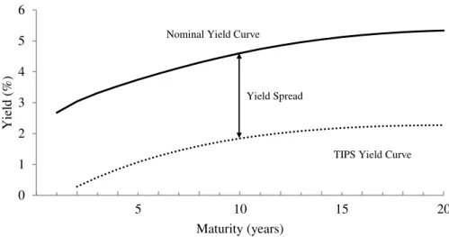
Figure 1: Nominal and TIPS yield curve of 2/12/2004 .
This relation can be represented graphically:
For the date of 2/12/2004, the yield spread between nominal and indexed bonds
maturing in 10 years is . This can be interpreted as follows: for a
maturity of 10 years a nominal bond offers investors a yield of , a TIPS offers
investors a yield of and the expected average annual inflation between 2/12/2004
and the 2/12/2014 is percentage points . From the definition of breakeven inflation
(BEI) stated in section 1, we can also think of as the level of average annual
inflation that, if realized, would offer the same return to investors in TIPS and investors
in nominal bonds.
The Fisher relation, despite being a good approximation, does not hold necessarily
due to the lower liquidity of TIPS and the inflation risks incurred by investors of
nominal securities. To compensate them for these risks, investors require a premium in
the yields: investors in nominal securities require an inflation premium ( ) to 0
1 2 3 4 5 6
5 10 15 20
Yield
(
%)
Maturity (years)
Yield Spread Nominal Yield Curve
9
compensate them for the possibility of realized inflation being high enough to
significantly decrease their real gains; TIPS investors require a liquidity premium ( )
to compensate them for the lower liquidity of their securities in secondary markets.
Taking these premia into account, the yield spread can be decomposed into the expected
inflation , the inflation premium and the liquidity premium :
.
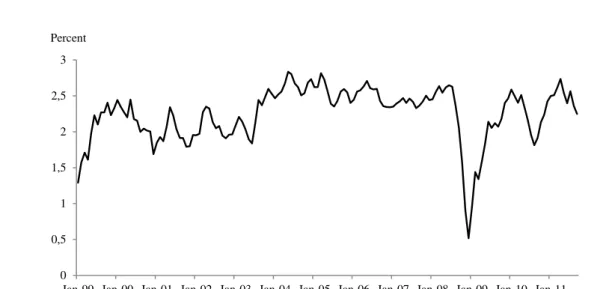
According to Gurkaynak et al. (2008) “this estimated liquidity premium is high, but it is
also very inertial” and it “remained big in the early years and then gradually faded away
in 2003.” Estimates by Pericoli (2012) suggest a small risk premium in the initial years
of the TIPS market and a considerable and variable inflation risk premium from 2001
onwards. Consequently, despite expected inflation being the main component of the
yield spread, the liquidity and inflation risk premia are significant and breakeven
inflation rates should not be directly interpreted as the market’s expectation of average
inflation.
0 0,5 1 1,5 2 2,5 3
Jan-99 Jan-00 Jan-01 Jan-02 Jan-03 Jan-04 Jan-05 Jan-06 Jan-07 Jan-08 Jan-09 Jan-10 Jan-11 Percent
10
4 Methodology
In this work project we constructed pseudo out-of-sample forecasts of month-on-month
inflation based on the TIPS yield curve by using breakeven inflation series with
different maturities as additional regressors in simple autoregressive models.
Comparing these forecasts to those of simple autoregressive processes we can assess the
value added of the market expectations of inflation in forecasts of inflation. We
forecasted the evolution of CPI at various horizons up to 2 years and computed
quarterly inflation forecasts comparing them to SPF median forecasts.
4.1 Data
As stated in section 3.2, the data of the TIPS yield curve was computed by Refet S.
Gurkaynak, Brian Sack, and Jonathan H. Wright with the methodology explained in
Gurkaynak et al. (2008) and downloaded from the Research Data section of the Board
of Governors of the Federal Reserve System’s webpage.6 This data set includes real yields and breakeven inflation rates expressed in various types of debt securities
(zero-coupon, par, instantaneous forward, one-year forward, five-to-ten-year forward) and
collected daily between January of 1999 and September of 2011. We opted to use
zero-coupon breakeven inflation series with maturities of 5, 6,..., 19 and 20 years and
converted the daily data to month-on-month data using simple averages. 7
Realized inflation was computed using logarithmic changes in non-seasonally
adjusted consumer price index for all urban consumers (CPI-U) downloaded from the
Bureau of Labor Statistics of the U.S. Department of Labor webpage8.
6
The data set is updated on a weekly basis.
7
There are breakeven inflation series with maturities of 2, 3 and 4 years but they are only available from 2004 onwards.
8
11
The forecasts of SPF were downloaded from the Federal Reserve of Philadelphia
webpage9.
4.2 Forecasts
4.2.1 Month-on-month inflation forecasts
Month-on-month inflation was forecasted using the following methods:
1. Direct autoregression (DAR) with forecast horizon h and p lags:
∑
where is inflation at and is the regression error. The number of
lags can be fixed (FL) or determined by the Akaike Information Criterion (AIC).
2. Iterated autoregression (IAR) forecasts with forecasting horizon h and p lags:
∑
and
̂ ̂ ∑ ̂ ̂ where ̂ for
̂ is the forecast of inflation at computed using past inflation for
and forecasts for . The lag length can be fixed (FL), determined by the
Akaike Information Criterion (AIC) or determined by the Bayes Information
Criterion (BIC).
3. Direct augmented auto regression (DAAR) with forecasting horizon h and p
lags:
∑
∑ ∑
The lag length is determined by the Akaike Information Criterion (AIC).
9
12
4. No-change forecast:
for any horizon h.
Forecasts computed with these methods were performed with
periods, fixed number of lags or maximum number of lags
. In order to avoid erroneous results due to lack of sufficient
observations to produce forecasts with long horizons three evaluation periods (defined
the starting observation (SO) parameter) were used for this pseudo out-of-sample
forecasts: February of 2002 until September of 2011( ; February of 2003 to
September of 2011 ; February of 2004 to September of 2011 , only
for forecasts with ).
4.2.2 Quarterly inflation forecasts and comparison with SPF
The SPF is performed every quarter by a small group of professional forecasters who
answer a survey elaborated by the Federal Reserve Bank of Philadelphia during the
middle month of each quarter. Their individual answers are collected and statistically
treated to obtain mean and median forecasts of various macroeconomic variables for the
current and following five quarters. One of the forecasted variables is quarterly
inflation, defined as percentage changes instead of logarithmic differences (Ang et al.
(2007)) of the average quarterly levels of the seasonally adjusted CPI-U.
To produce quarterly inflation forecasts comparable to SPF forecasts we first
forecasted month-on-month inflation with two methods: the Iterated Autoregression
13
inflation included in the TIPS yield curve we as additional regressors (we used all the
breakeven inflation series with maturities ranging from 5 to 20 years). Month-on-month
inflation was forecasted with and the maximum number of lags of 6.
We then used these results to forecast the evolution of the seasonally adjusted CPI-U
over the following 11 months after the initial month of each quarter. For example, in the
first quarter of 2002 (2002:Q1), information of past inflation and of expected future
inflation extracted from the TIPS yield curve available until January of 2002 was used
to forecast February’s inflation ( ̂ ), March’s inflation ( ̂ ) and the inflation for
the following months until December ( ̂ . In order to make a fair comparison
between our methodology and the SPF we took into account the fact that when
professional forecasters answer the survey during the middle month of the quarter the
CPI of the first month of that quarter is already known. Therefore, we used the actual
value of the CPI of the first month of each quarter and the forecast of inflation
for the second month of the quarter ̂ to forecast the CPI of the second month of
that quarter:
̂ ̂
The forecast of ̂ was used to forecast the price level of the third month of that
quarter:
̂ ̂ ̂
This recursive procedure was iterated to forecast the CPI level for the following months
( ̂ , ̂ , …, ̂ . The actual CPI and the forecasted levels of CPI were
converted into quarterly (as 3-month averages) data. This procedure was performed for
the period between 2002Q1 and 2011Q2. Our forecasts directly comparable to the
14
5 Results
5.1 Month-on-month inflation
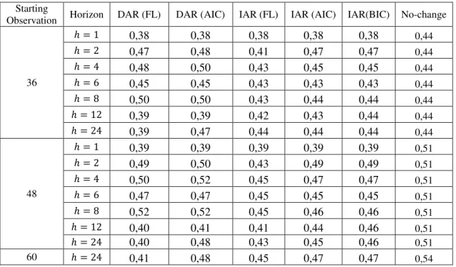
Forecasts of month-on-month inflation (measured as logarithmic changes of the
non-seasonally adjusted CPI-U) produced using the methods presented in section 4.2.1 were
evaluated using the root mean square forecasting error (RMSFE).10 For each of the simple autoregressive methods used (DAR (FL), DAR (AIC), IAR (FL), IAR (AIC) and
IAR (BIC)) we constructed a benchmark by choosing the forecasts for each horizon and
starting observation with the lag length corresponding to the smallest RMSFE.
Forecasts from DAAR (AIC) using breakeven inflation series as additional regressors
were compared to these benchmarks to infer the added value of incorporating
expectations of future inflation as additional regressors to simple autoregressive
forecasting methods.
Starting
Observation Horizon DAR (FL) DAR (AIC) IAR (FL) IAR (AIC) IAR(BIC) No-change
36
0,38 0,38 0,38 0,38 0,38 0,44
0,47 0,48 0,41 0,47 0,47 0,44
0,48 0,50 0,43 0,45 0,45 0,44
0,45 0,45 0,43 0,43 0,43 0,44
0,50 0,50 0,43 0,44 0,44 0,44
0,39 0,39 0,42 0,43 0,44 0,44
0,39 0,47 0,44 0,44 0,44 0,44
48
0,39 0,39 0,39 0,39 0,39 0,51
0,49 0,50 0,43 0,49 0,49 0,51
0,50 0,52 0,45 0,47 0,47 0,51
0,47 0,47 0,45 0,45 0,45 0,51
0,52 0,52 0,45 0,46 0,46 0,51
0,40 0,41 0,41 0,44 0,46 0,51
0,40 0,48 0,43 0,45 0,46 0,51
60 0,41 0,48 0,45 0,47 0,47 0,54
10
∑ ̂ where ̂ is the forecast of .
15
From table 1 we can conclude that the IAR (FL) is the best benchmark forecasting
method used in this exercise. Therefore, until the end of this section we will treat the
IAR (FL) method as the global benchmark and present the forecasting errors as relative
RMSFE, defined as, for a given horizon, the ratio of the RMSFE of the forecasting
method and the RMSFE of IAR (FL).
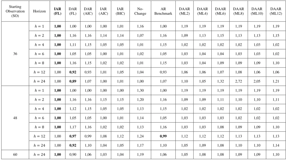
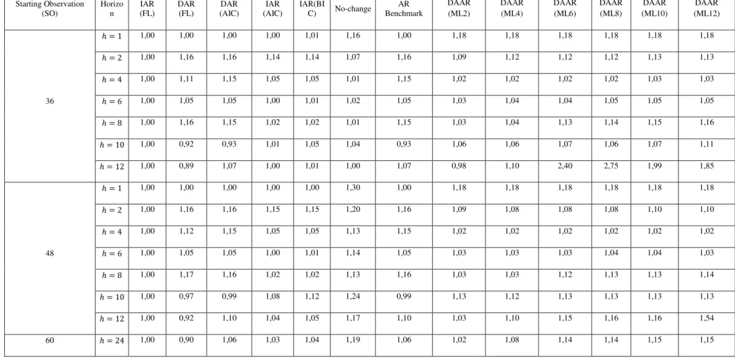
In table 2 we present the relative RMSFE of month-on-month inflation forecasts of the
simple autoregressive methods and the augmented autoregressive forecasts using the
breakeven inflation series with maturity of 10 years as an additional regressor. 11For each horizon within each evaluation period (defined by the SO) the lowest relative
RMSFE is highlighted in bold. From table 2 we conclude that, despite not having lower
RMSFE than the benchmark IAR (FL) for any of the horizons and evaluation periods
used, the DAAR forecasts improve simple univariate forecasts (AR Benchmark) for
horizons of 2, 4 and 8 periods and have very similar RMSFE than the benchmark
method IAR (FL) for forecast horizons of 2, 4, 6 and 8 periods, in the two main
evaluation periods (SO=36 and SO=48), unlike the No-change method in the first
evaluation period (SO=36). Taking into account these consistently similar results to
those of the benchmark method IAR (FL) for these horizons and the fact that these
benchmarks of simple autoregressive methods were artificially created choosing for
each horizon the forecasts with the lowest RMSFE of various forecasts that differ in the
number of lags, we decided that the DAAR method using inflation expectations
extracted from the TIPS yield curve can provide worthy forecasts of month-on-month
inflation to forecast quarterly inflation with the method explained in section 4.2.2.
11
16 DAAR (ML12) 1,19 1,15 1,02 1,02 1,10 1,06 1,21 1,19 1,11 1,02 1,02 1,10 1,13 1,14 1,10 DAAR (ML10) 1,19 1,13 1,03 1,03 1,09 1,06 2,05 1,19 1,10 1,02 1,02 1,09 1,13 1,10 1,09 DAAR (ML8) 1,19 1,13 1,02 1,03 1,09 1,08 2,72 1,19 1,10 1,02 1,02 1,09 1,13 1,10 1,09 DAAR (ML6) 1,19 1,15 1,02 1,04 1,09 1,07 1,32 1,19 1,11 1,02 1,03 1,08 1,12 1,08 1,08 DAAR (ML4) 1,19 1,13 1,02 1,04 1,04 1,06 1,05 1,19 1,09 1,02 1,03 1,03 1,12 1,09 1,08 DAAR (ML2) 1,19 1,09 1,02 1,03 1,03 1,06 1,10 1,19 1,09 1,02 1,03 1,03 1,12 1,05 1,05 AR Benchmark 1,00 1,16 1,15 1,05 1,15 0,93 1,07 1,00 1,16 1,15 1,05 1,16 0,99 1,10 1,06 No-Change 1,16 1,07 1,01 1,02 1,01 1,04 1,00 1,30 1,20 1,13 1,14 1,13 1,24 1,17 1,19 IAR (BIC) 1,01 1,14 1,05 1,01 1,02 1,05 1,01 1,00 1,15 1,05 1,01 1,02 1,12 1,05 1,04 IAR (AIC) 1,00 1,14 1,05 1,00 1,02 1,01 1,00 1,00 1,15 1,05 1,00 1,02 1,08 1,04 1,03 DAR (AIC) 1,00 1,16 1,15 1,05 1,15 0,93 1,07 1,00 1,16 1,15 1,05 1,16 0,99 1,10 1,06 DAR (FL) 1,00 1,16 1,11 1,05 1,16 0,92 0,89 1,00 1,16 1,12 1,05 1,17 0,97 0,92 0,90 IAR (FL) 1,00 1,00 1,00 1,00 1,00 1,00 1,00 1,00 1,00 1,00 1,00 1,00 1,00 1,00 1,00 Horizon Starting Observation (SO) 36 48 60
17
5.2 Quarterly inflation forecasts
Quarterly inflation was forecasted with (a forecasting horizon of 1 period
corresponds to the quarter during which the SPF is performed). As in the previous
forecasting exercise, inflation forecasts using different breakeven inflation series
yielded very similar results but the series with maturities of 5 and 7 years provided the
best TIPS based forecasts of quarterly inflation. The relative RMSFE of the best
forecasts of quarterly inflation are presented in the following table:
Forecast horizon
SPF 1,97 1,15 1,13 1,13
IAR (FL1) 1,00 1,00 1,03 1,04
IAR (FL2) 1,13 1,08 1,03 1,04
TIPS based (BEI05Y) 1,19 1,02 1,00 1,00
TIPS based (BEI07Y) 1,16 1,02 1,01 1,00
The superior results of the IAR (FL) forecasts for confirms the superior results of
this autoregressive model for forecasting month-on-month inflation for short horizons
expressed in tables 1 and 2. However, for horizons of 3 and 4 periods forecasts
computed with inflation expectations extracted from the TIPS yield curve obtained the
best results, proving their worthiness in forecasting month-on-month inflation with
horizons between 6 and 11 periods. Both of these methods were able to beat the SPF
forecasts for every horizon.
6 Conclusions
In this work project we have shown that using breakeven inflation series as additional
regressors to simple autoregressive processes can improve forecasts of month-on-month
18
forecasts based on inflation expectations are very close to those of forecasts produced
with the best method tested (iterated autoregression with fixed lag length).
Quarterly inflation forecasts derived from month-on-month inflation forecasts computed
with a fixed lag iterated autoregressive method outperformed the SPF for horizons of 1
and 2 periods. On the other hand, forecasts backed by inflation expectations extracted
from the TIPS yield curve outperformed SPF for horizons of 3 and 4 periods.
Estimating liquidity and inflation risk premiums would provide a more accurate
measure of expected inflation than breakeven inflation series and using them as
additional regressors should improve the forecasts performed in this work project. This
would be of considerable importance in the case of month-on-month inflation forecasts
as they are slightly outperformed by iterated autoregressive with fixed lag length.
References
Ang, A, Bekaert, G. and Wei, M. 2007. “Do macro variables, asset markets, or
surveys forecast inflation better?” Journal of Monetary Economics, Vol. 54, pages 1163-1212.
D’Amico, S., Kim, D., Wei, M. 2008. “Tips from TIPS: the informational content of Treasury Inflation - Protected Security prices”. Bank of International Settlements, Working Paper 248
Dudley, W.C., Roush, J., and Ezer, M.S. 2009. “The Case for TIPS: An Examination
19
Gurkaynak, R.S., Sack, B. and Wright, J. H. 2007. “The U.S. Treasury Yield Curve:
1961 to the Present”,Journal of Monetary Economics, Elsevier, vol. 54(8), pages 2291-2304, November.
Gurkaynak, R.S., Sack, B. and Wright, J. H. 2010. "The TIPS Yield Curve and
Inflation Compensation." American Economic Journal: Macroeconomics, American Economic Association, vol. 2(1), pages 70-92, January
Pericoli, M. 2012 “Expected inflation and inflation risk premium in the euro area and in
the United States”, Bank of Italy Working Paper number 842
Shen, Pu. 2009. “Developing a liquid market for inflation-indexed government
securities: lessons from earlier experiences”, Federal Reserve Bank of Kansas City Economic Review, first quarter, pages 89-113.
Shen, P. and Corning, J. 2001. “Can TIPS Help Identify Long-Term Inflation
Expectations?” Federal Reserve Bank of Kansas City Economic Review, fourth quarter, pages 61-87.
Stock, J. H., and Watson, M. W. 2007. “Why Has U.S. Inflation Become Harder to
Forecast?” Journal of Money, Credit and Banking 39(1): 3–34.
Stock, J. H., and Watson, M. W. 2008. “Phillips Curve Inflation Forecasts.” National
20
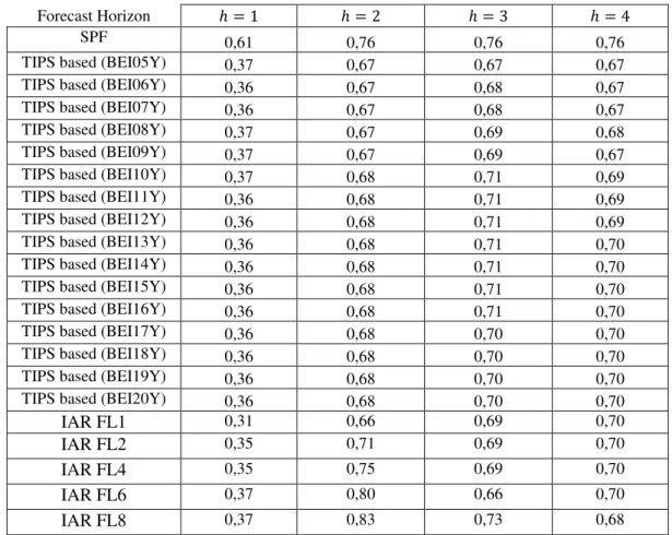
Appendix A
–
RMSFE of Quarterly Inflation Forecasts
Forecast Horizon
SPF 0,61 0,76 0,76 0,76
TIPS based (BEI05Y) 0,37 0,67 0,67 0,67
TIPS based (BEI06Y) 0,36 0,67 0,68 0,67
TIPS based (BEI07Y) 0,36 0,67 0,68 0,67
TIPS based (BEI08Y) 0,37 0,67 0,69 0,68
TIPS based (BEI09Y) 0,37 0,67 0,69 0,67
TIPS based (BEI10Y) 0,37 0,68 0,71 0,69
TIPS based (BEI11Y) 0,36 0,68 0,71 0,69
TIPS based (BEI12Y) 0,36 0,68 0,71 0,69
TIPS based (BEI13Y) 0,36 0,68 0,71 0,70
TIPS based (BEI14Y) 0,36 0,68 0,71 0,70
TIPS based (BEI15Y) 0,36 0,68 0,71 0,70
TIPS based (BEI16Y) 0,36 0,68 0,71 0,70
TIPS based (BEI17Y) 0,36 0,68 0,70 0,70
TIPS based (BEI18Y) 0,36 0,68 0,70 0,70
TIPS based (BEI19Y) 0,36 0,68 0,70 0,70
TIPS based (BEI20Y) 0,36 0,68 0,70 0,70
IAR FL1 0,31 0,66 0,69 0,70
IAR FL2 0,35 0,71 0,69 0,70
IAR FL4 0,35 0,75 0,69 0,70
IAR FL6 0,37 0,80 0,66 0,70
IAR FL8 0,37 0,83 0,73 0,68
21
Appendix B
–
Relative RMSFE of Month-onMonth forecasts
Table 5 -Relative RMSFE of month-on-month inflation forecasts produced with benchmark autoregressive methods and direct augmented autoregressive forecasts with breakeven inflation with maturity of 7 years (MLX denotes the number of maximum lags parameter of AIC lag length selection in DAAR method)
Starting Observation
(SO) Horizon IAR (FL) DAR (FL) DAR (AIC) IAR (AIC) IAR(BIC) No-change
AR Benchmark
DAAR (ML2)
DAAR (ML4)
DAAR (ML6)
DAAR (ML8)
DAAR (ML10)
DAAR (ML12)
36
1,00 1,00 1,00 1,00 1,01 1,16 1,00 1,18 1,18 1,18 1,19 1,19 1,19
1,00 1,16 1,16 1,14 1,14 1,07 1,16 1,09 1,13 1,13 1,14 1,13 1,13
1,00 1,11 1,15 1,05 1,05 1,01 1,15 1,02 1,02 1,02 1,03 1,03 1,02
1,00 1,05 1,05 1,00 1,01 1,02 1,05 1,03 1,03 1,03 1,05 1,05 1,05
1,00 1,16 1,15 1,02 1,02 1,01 1,15 1,04 1,04 1,15 1,15 1,16 1,18
1,00 0,92 0,93 1,01 1,05 1,04 0,93 1,06 1,06 1,07 1,06 1,07 1,11
1,00 0,89 1,07 1,00 1,01 1,00 1,07 0,98 1,11 1,81 4,75 2,28 1,84
48
1,00 1,00 1,00 1,00 1,00 1,30 1,00 1,17 1,18 1,18 1,19 1,19 1,19
1,00 1,16 1,16 1,15 1,15 1,20 1,16 1,09 1,09 1,09 1,10 1,10 1,10
1,00 1,12 1,15 1,05 1,05 1,13 1,15 1,03 1,02 1,02 1,03 1,02 1,02
1,00 1,05 1,05 1,00 1,01 1,14 1,05 1,03 1,03 1,03 1,03 1,03 1,04
1,00 1,17 1,16 1,02 1,02 1,13 1,16 1,03 1,03 1,14 1,14 1,15 1,16
1,00 0,97 0,99 1,08 1,12 1,24 0,99 1,13 1,12 1,13 1,13 1,13 1,13
1,00 0,92 1,10 1,04 1,05 1,17 1,10 1,02 1,11 1,17 1,18 1,18 1,55
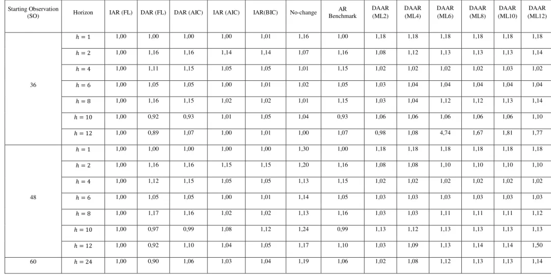
Table 6 -Relative RMSFE of month-on-month inflation forecasts produced with benchmark autoregressive methods and direct augmented autoregressive forecasts with breakeven inflation with maturity of 6 years (MLX denotes the number of maximum lags parameter of AIC lag length selection in DAAR method)
Starting Observation (SO)
Horizo n
IAR (FL)
DAR (FL)
DAR (AIC)
IAR (AIC)
IAR(BI
C) No-change
AR Benchmark
DAAR (ML2)
DAAR (ML4)
DAAR (ML6)
DAAR (ML8)
DAAR (ML10)
DAAR (ML12)
36
1,00 1,00 1,00 1,00 1,01 1,16 1,00 1,18 1,18 1,18 1,18 1,18 1,18
1,00 1,16 1,16 1,14 1,14 1,07 1,16 1,09 1,12 1,12 1,12 1,13 1,13
1,00 1,11 1,15 1,05 1,05 1,01 1,15 1,02 1,02 1,02 1,02 1,03 1,03
1,00 1,05 1,05 1,00 1,01 1,02 1,05 1,03 1,04 1,04 1,05 1,05 1,05
1,00 1,16 1,15 1,02 1,02 1,01 1,15 1,03 1,04 1,13 1,14 1,15 1,16
1,00 0,92 0,93 1,01 1,05 1,04 0,93 1,06 1,06 1,07 1,06 1,07 1,11
1,00 0,89 1,07 1,00 1,01 1,00 1,07 0,98 1,10 2,40 2,75 1,99 1,85
48
1,00 1,00 1,00 1,00 1,00 1,30 1,00 1,18 1,18 1,18 1,18 1,18 1,18
1,00 1,16 1,16 1,15 1,15 1,20 1,16 1,09 1,08 1,08 1,08 1,10 1,10
1,00 1,12 1,15 1,05 1,05 1,13 1,15 1,02 1,02 1,02 1,02 1,02 1,02
1,00 1,05 1,05 1,00 1,01 1,14 1,05 1,03 1,03 1,03 1,04 1,04 1,03
1,00 1,17 1,16 1,02 1,02 1,13 1,16 1,03 1,03 1,12 1,13 1,13 1,14
1,00 0,97 0,99 1,08 1,12 1,24 0,99 1,13 1,12 1,13 1,13 1,13 1,13
1,00 0,92 1,10 1,04 1,05 1,17 1,10 1,03 1,10 1,15 1,16 1,16 1,54
Table 7 -Relative RMSFE of month-on-month inflation forecasts produced with benchmark autoregressive methods and direct augmented autoregressive forecasts with breakeven inflation with maturity of 7 years (MLX denotes the number of maximum lags parameter of AIC lag length selection in DAAR method)
Starting Observation
(SO) Horizon IAR (FL) DAR (FL) DAR (AIC) IAR (AIC) IAR(BIC) No-change
AR Benchmark
DAAR (ML2)
DAAR (ML4)
DAAR (ML6)
DAAR (ML8)
DAAR (ML10)
DAAR (ML12)
36
1,00 1,00 1,00 1,00 1,01 1,16 1,00 1,18 1,18 1,18 1,18 1,18 1,18
1,00 1,16 1,16 1,14 1,14 1,07 1,16 1,08 1,12 1,13 1,13 1,13 1,14
1,00 1,11 1,15 1,05 1,05 1,01 1,15 1,02 1,02 1,02 1,02 1,03 1,02
1,00 1,05 1,05 1,00 1,01 1,02 1,05 1,03 1,04 1,04 1,04 1,04 1,04
1,00 1,16 1,15 1,02 1,02 1,01 1,15 1,03 1,04 1,12 1,12 1,13 1,14
1,00 0,92 0,93 1,01 1,05 1,04 0,93 1,06 1,06 1,06 1,06 1,06 1,10
1,00 0,89 1,07 1,00 1,01 1,00 1,07 0,98 1,08 4,74 1,67 1,81 1,77
48
1,00 1,00 1,00 1,00 1,00 1,30 1,00 1,18 1,18 1,18 1,18 1,18 1,18
1,00 1,16 1,16 1,15 1,15 1,20 1,16 1,08 1,08 1,10 1,10 1,10 1,10
1,00 1,12 1,15 1,05 1,05 1,13 1,15 1,02 1,02 1,02 1,02 1,02 1,02
1,00 1,05 1,05 1,00 1,01 1,14 1,05 1,03 1,03 1,03 1,03 1,03 1,03
1,00 1,17 1,16 1,02 1,02 1,13 1,16 1,03 1,03 1,11 1,11 1,11 1,12
1,00 0,97 0,99 1,08 1,12 1,24 0,99 1,13 1,12 1,13 1,13 1,13 1,13
1,00 0,92 1,10 1,04 1,05 1,17 1,10 1,03 1,09 1,13 1,14 1,14 1,50
Table 8 -Relative RMSFE of month-on-month inflation forecasts produced with benchmark autoregressive methods and direct augmented autoregressive forecasts with breakeven inflation with a maturity of 8 years (MLX denotes the number of maximum lags parameter of AIC lag length selection in DAAR method)
Starting Observation
(SO) Horizon IAR (FL) DAR (FL) DAR (AIC) IAR (AIC) IAR(BIC) No-change
AR Benchmark
DAAR (ML2)
DAAR (ML4)
DAAR (ML6)
DAAR (ML8)
DAAR (ML10)
DAAR (ML12)
36
1,00 1,00 1,00 1,00 1,01 1,16 1,00 1,18 1,18 1,18 1,18 1,19 1,18
1,00 1,16 1,16 1,14 1,14 1,07 1,16 1,09 1,12 1,14 1,14 1,14 1,14
1,00 1,11 1,15 1,05 1,05 1,01 1,15 1,02 1,02 1,02 1,02 1,04 1,02
1,00 1,05 1,05 1,00 1,01 1,02 1,05 1,03 1,04 1,04 1,04 1,04 1,03
1,00 1,16 1,15 1,02 1,02 1,01 1,15 1,03 1,04 1,10 1,11 1,11 1,12
1,00 0,92 0,93 1,01 1,05 1,04 0,93 1,06 1,06 1,07 1,06 1,06 1,11
1,00 0,89 1,07 1,00 1,01 1,00 1,07 0,99 1,07 6,52 1,42 1,68 2,17
48
1,00 1,00 1,00 1,00 1,00 1,30 1,00 1,18 1,18 1,18 1,18 1,19 1,18
1,00 1,16 1,16 1,15 1,15 1,20 1,16 1,09 1,08 1,10 1,10 1,10 1,10
1,00 1,12 1,15 1,05 1,05 1,13 1,15 1,02 1,02 1,02 1,02 1,02 1,02
1,00 1,05 1,05 1,00 1,01 1,14 1,05 1,03 1,03 1,03 1,03 1,03 1,02
1,00 1,17 1,16 1,02 1,02 1,13 1,16 1,03 1,03 1,10 1,10 1,10 1,11
1,00 0,97 0,99 1,08 1,12 1,24 0,99 1,12 1,12 1,13 1,13 1,13 1,13
1,00 0,92 1,10 1,04 1,05 1,17 1,10 1,04 1,09 1,12 1,12 1,13 1,84
Table 9 -Relative RMSFE of month-on-month inflation forecasts produced with benchmark autoregressive methods and direct augmented autoregressive forecasts with breakeven inflation with maturity of 9 years (MLX denotes the number of maximum lags parameter of AIC lag length selection in DAAR method)
Starting Observation
(SO) Horizon IAR (FL) DAR (FL) DAR (AIC) IAR (AIC) IAR(BIC) No-change
AR Benchmark
DAAR (ML2)
DAAR (ML4)
DAAR (ML6)
DAAR (ML8)
DAAR (ML10)
DAAR (ML12)
36
1,00 1,00 1,00 1,00 1,01 1,16 1,00 1,19 1,19 1,19 1,18 1,18 1,18
1,00 1,16 1,16 1,14 1,14 1,07 1,16 1,09 1,12 1,13 1,13 1,14 1,14
1,00 1,11 1,15 1,05 1,05 1,01 1,15 1,02 1,02 1,02 1,02 1,04 1,02
1,00 1,05 1,05 1,00 1,01 1,02 1,05 1,03 1,04 1,04 1,03 1,03 1,03
1,00 1,16 1,15 1,02 1,02 1,01 1,15 1,03 1,04 1,09 1,10 1,10 1,11
1,00 0,92 0,93 1,01 1,05 1,04 0,93 1,06 1,06 1,07 1,06 1,06 1,05
1,00 0,89 1,07 1,00 1,01 1,00 1,07 1,00 1,06 1,89 1,48 1,59 10,09
48
1,00 1,00 1,00 1,00 1,00 1,30 1,00 1,19 1,19 1,20 1,18 1,18 1,19
1,00 1,16 1,16 1,15 1,15 1,20 1,16 1,09 1,08 1,10 1,10 1,10 1,10
1,00 1,12 1,15 1,05 1,05 1,13 1,15 1,02 1,02 1,02 1,02 1,02 1,02
1,00 1,05 1,05 1,00 1,01 1,14 1,05 1,03 1,03 1,03 1,02 1,02 1,02
1,00 1,17 1,16 1,02 1,02 1,13 1,16 1,03 1,03 1,09 1,09 1,09 1,10
1,00 0,97 0,99 1,08 1,12 1,24 0,99 1,12 1,12 1,13 1,13 1,13 1,13
1,00 0,92 1,10 1,04 1,05 1,17 1,10 1,04 1,09 1,10 1,10 1,11 1,13
Table 10 -Relative RMSFE of month-on-month inflation forecasts produced with benchmark autoregressive methods and direct augmented autoregressive forecasts with breakeven inflation with maturity of 10 years (MLX denotes the number of maximum lags parameter of AIC lag length selection in DAAR method)
Starting Observation
(SO) Horizon IAR (FL) DAR (FL) DAR (AIC) IAR (AIC) IAR(BIC) No-change
AR Benchmark
DAAR (ML2)
DAAR (ML4)
DAAR (ML6)
DAAR (ML8)
DAAR (ML10)
DAAR (ML12)
36
1,00 1,00 1,00 1,00 1,01 1,16 1,00 1,19 1,19 1,19 1,19 1,19 1,19
1,00 1,16 1,16 1,14 1,14 1,07 1,16 1,09 1,13 1,15 1,13 1,13 1,15
1,00 1,11 1,15 1,05 1,05 1,01 1,15 1,02 1,02 1,02 1,02 1,03 1,02
1,00 1,05 1,05 1,00 1,01 1,02 1,05 1,03 1,04 1,04 1,03 1,03 1,02
1,00 1,16 1,15 1,02 1,02 1,01 1,15 1,03 1,04 1,09 1,09 1,09 1,10
1,00 0,92 0,93 1,01 1,05 1,04 0,93 1,06 1,06 1,07 1,08 1,06 1,06
1,00 0,89 1,07 1,00 1,01 1,00 1,07 1,10 1,05 1,32 2,72 2,05 1,21
48
1,00 1,00 1,00 1,00 1,00 1,30 1,00 1,19 1,19 1,19 1,19 1,19 1,19
1,00 1,16 1,16 1,15 1,15 1,20 1,16 1,09 1,09 1,11 1,10 1,10 1,11
1,00 1,12 1,15 1,05 1,05 1,13 1,15 1,02 1,02 1,02 1,02 1,02 1,02
1,00 1,05 1,05 1,00 1,01 1,14 1,05 1,03 1,03 1,03 1,02 1,02 1,02
1,00 1,17 1,16 1,02 1,02 1,13 1,16 1,03 1,03 1,08 1,09 1,09 1,10
1,00 0,97 0,99 1,08 1,12 1,24 0,99 1,12 1,12 1,12 1,13 1,13 1,13
1,00 0,92 1,10 1,04 1,05 1,17 1,10 1,05 1,09 1,08 1,10 1,10 1,14
Table 11 -Relative RMSFE of month-on-month inflation forecasts produced with benchmark autoregressive methods and direct augmented autoregressive forecasts with breakeven inflation with maturity of 11 years (MLX denotes the number of maximum lags parameter of AIC lag length selection in DAAR method)
Starting Observation
(SO) Horizon IAR (FL) DAR (FL) DAR (AIC) IAR (AIC) IAR(BIC) No-change
AR Benchmark
DAAR (ML2)
DAAR (ML4)
DAAR (ML6)
DAAR (ML8)
DAAR (ML10)
DAAR (ML12)
36
1,00 1,00 1,00 1,00 1,01 1,16 1,00 1,18 1,19 1,19 1,19 1,19 1,19
1,00 1,16 1,16 1,14 1,14 1,07 1,16 1,09 1,13 1,15 1,15 1,15 1,15
1,00 1,11 1,15 1,05 1,05 1,01 1,15 1,02 1,02 1,02 1,02 1,03 1,02
1,00 1,05 1,05 1,00 1,01 1,02 1,05 1,03 1,04 1,04 1,04 1,03 1,05
1,00 1,16 1,15 1,02 1,02 1,01 1,15 1,04 1,04 1,08 1,07 1,07 1,10
1,00 0,92 0,93 1,01 1,05 1,04 0,93 1,05 1,06 1,07 1,09 1,11 1,09
1,00 0,89 1,07 1,00 1,01 1,00 1,07 1,01 1,05 1,15 2,22 3,64 1,24
48
1,00 1,00 1,00 1,00 1,00 1,30 1,00 1,19 1,19 1,19 1,19 1,20 1,19
1,00 1,16 1,16 1,15 1,15 1,20 1,16 1,09 1,09 1,11 1,11 1,11 1,11
1,00 1,12 1,15 1,05 1,05 1,13 1,15 1,02 1,02 1,02 1,02 1,02 1,02
1,00 1,05 1,05 1,00 1,01 1,14 1,05 1,03 1,03 1,04 1,04 1,02 1,05
1,00 1,17 1,16 1,02 1,02 1,13 1,16 1,03 1,04 1,07 1,07 1,07 1,10
1,00 0,97 0,99 1,08 1,12 1,24 0,99 1,12 1,12 1,12 1,13 1,13 1,13
1,00 0,92 1,10 1,04 1,05 1,17 1,10 1,06 1,08 1,08 1,09 1,09 1,15
Table 12 -Relative RMSFE of month-on-month inflation forecasts produced with benchmark autoregressive methods and direct augmented autoregressive forecasts with breakeven inflation with maturity of 12 years (MLX denotes the number of maximum lags parameter of AIC lag length selection in DAAR method)
Starting Observation
(SO) Horizon IAR (FL) DAR (FL) DAR (AIC) IAR (AIC) IAR(BIC) No-change
AR Benchmark
DAAR (ML2)
DAAR (ML4)
DAAR (ML6)
DAAR (ML8)
DAAR (ML10)
DAAR (ML12)
36
1,00 1,00 1,00 1,00 1,01 1,16 1,00 1,18 1,18 1,18 1,19 1,19 1,19
1,00 1,16 1,16 1,14 1,14 1,07 1,16 1,09 1,13 1,15 1,14 1,15 1,15
1,00 1,11 1,15 1,05 1,05 1,01 1,15 1,02 1,02 1,02 1,02 1,03 1,02
1,00 1,05 1,05 1,00 1,01 1,02 1,05 1,03 1,04 1,04 1,05 1,05 1,05
1,00 1,16 1,15 1,02 1,02 1,01 1,15 1,03 1,04 1,06 1,07 1,07 1,10
1,00 0,92 0,93 1,01 1,05 1,04 0,93 1,05 1,05 1,07 1,09 1,10 1,14
1,00 0,89 1,07 1,00 1,01 1,00 1,07 1,02 1,05 1,09 4,05 43,97 1,10
48
1,00 1,00 1,00 1,00 1,00 1,30 1,00 1,19 1,19 1,19 1,19 1,19 1,19
1,00 1,16 1,16 1,15 1,15 1,20 1,16 1,09 1,09 1,11 1,11 1,11 1,11
1,00 1,12 1,15 1,05 1,05 1,13 1,15 1,02 1,02 1,02 1,02 1,02 1,02
1,00 1,05 1,05 1,00 1,01 1,14 1,05 1,03 1,04 1,04 1,05 1,05 1,05
1,00 1,17 1,16 1,02 1,02 1,13 1,16 1,03 1,03 1,06 1,06 1,06 1,09
1,00 0,97 0,99 1,08 1,12 1,24 0,99 1,12 1,12 1,12 1,13 1,13 1,13
1,00 0,92 1,10 1,04 1,05 1,17 1,10 1,06 1,08 1,08 1,08 1,08 1,10
Table 13 -Relative RMSFE of month-on-month inflation forecasts produced with benchmark autoregressive methods and direct augmented autoregressive forecasts with breakeven inflation with maturity of 13 years (MLX denotes the number of maximum lags parameter of AIC lag length selection in DAAR method)
Starting Observation
(SO) Horizon IAR (FL) DAR (FL) DAR (AIC) IAR (AIC) IAR(BIC) No-change
AR Benchmark
DAAR (ML2)
DAAR (ML4)
DAAR (ML6)
DAAR (ML8)
DAAR (ML10)
DAAR (ML12)
36
1,00 1,00 1,00 1,00 1,01 1,16 1,00 1,18 1,18 1,18 1,19 1,19 1,19
1,00 1,16 1,16 1,14 1,14 1,07 1,16 1,10 1,13 1,15 1,14 1,15 1,15
1,00 1,11 1,15 1,05 1,05 1,01 1,15 1,02 1,02 1,02 1,02 1,04 1,02
1,00 1,05 1,05 1,00 1,01 1,02 1,05 1,03 1,04 1,06 1,05 1,05 1,07
1,00 1,16 1,15 1,02 1,02 1,01 1,15 1,04 1,04 1,06 1,07 1,06 1,09
1,00 0,92 0,93 1,01 1,05 1,04 0,93 1,05 1,05 1,07 1,09 1,09 1,68
1,00 0,89 1,07 1,00 1,01 1,00 1,07 1,03 1,04 1,07 2,36 5,47 1,09
48
1,00 1,00 1,00 1,00 1,00 1,30 1,00 1,18 1,19 1,19 1,19 1,19 1,19
1,00 1,16 1,16 1,15 1,15 1,20 1,16 1,10 1,09 1,11 1,11 1,11 1,11
1,00 1,12 1,15 1,05 1,05 1,13 1,15 1,02 1,02 1,02 1,02 1,02 1,02
1,00 1,05 1,05 1,00 1,01 1,14 1,05 1,03 1,04 1,06 1,05 1,05 1,07
1,00 1,17 1,16 1,02 1,02 1,13 1,16 1,03 1,03 1,06 1,06 1,06 1,08
1,00 0,97 0,99 1,08 1,12 1,24 0,99 1,12 1,12 1,12 1,13 1,13 1,13
1,00 0,92 1,10 1,04 1,05 1,17 1,10 1,07 1,08 1,09 1,08 1,07 1,10
Table 14 -Relative RMSFE of month-on-month inflation forecasts produced with benchmark autoregressive methods and direct augmented autoregressive forecasts with breakeven inflation with maturity of 14 years (MLX denotes the number of maximum lags parameter of AIC lag length selection in DAAR method)
Starting Observation
(SO) Horizon IAR (FL) DAR (FL) DAR (AIC) IAR (AIC) IAR(BIC) No-change
AR Benchmark
DAAR (ML2)
DAAR (ML4)
DAAR (ML6)
DAAR (ML8)
DAAR (ML10)
DAAR (ML12)
36
1,00 1,00 1,00 1,00 1,01 1,16 1,00 1,18 1,18 1,18 1,19 1,19 1,19
1,00 1,16 1,16 1,14 1,14 1,07 1,16 1,10 1,13 1,15 1,14 1,15 1,15
1,00 1,11 1,15 1,05 1,05 1,01 1,15 1,02 1,02 1,02 1,02 1,04 1,03
1,00 1,05 1,05 1,00 1,01 1,02 1,05 1,04 1,04 1,06 1,07 1,06 1,07
1,00 1,16 1,15 1,02 1,02 1,01 1,15 1,03 1,04 1,06 1,06 1,06 1,08
1,00 0,92 0,93 1,01 1,05 1,04 0,93 1,05 1,05 1,07 1,09 1,09 2,20
1,00 0,89 1,07 1,00 1,01 1,00 1,07 1,03 1,05 1,06 1,39 5,95 1,06
48
1,00 1,00 1,00 1,00 1,00 1,30 1,00 1,18 1,19 1,19 1,19 1,19 1,19
1,00 1,16 1,16 1,15 1,15 1,20 1,16 1,10 1,09 1,11 1,11 1,11 1,11
1,00 1,12 1,15 1,05 1,05 1,13 1,15 1,02 1,02 1,02 1,02 1,02 1,02
1,00 1,05 1,05 1,00 1,01 1,14 1,05 1,03 1,03 1,06 1,07 1,06 1,07
1,00 1,17 1,16 1,02 1,02 1,13 1,16 1,03 1,03 1,05 1,05 1,06 1,08
1,00 0,97 0,99 1,08 1,12 1,24 0,99 1,12 1,12 1,12 1,13 1,13 1,13
1,00 0,92 1,10 1,04 1,05 1,17 1,10 1,08 1,09 1,08 1,09 1,07 1,07
Table 15 -Relative RMSFE of month-on-month inflation forecasts produced with benchmark autoregressive methods and direct augmented autoregressive forecasts with breakeven inflation with maturity of 15 years (MLX denotes the number of maximum lags parameter of AIC lag length selection in DAAR method)
Starting Observation
(SO) Horizon IAR (FL) DAR (FL) DAR (AIC) IAR (AIC) IAR(BIC) No-change
AR Benchmark
DAAR (ML2)
DAAR (ML4)
DAAR (ML6)
DAAR (ML8)
DAAR (ML10)
DAAR (ML12)
36
1,00 1,00 1,00 1,00 1,01 1,16 1,00 1,18 1,18 1,18 1,19 1,19 1,19
1,00 1,16 1,16 1,14 1,14 1,07 1,16 1,10 1,12 1,15 1,14 1,15 1,15
1,00 1,11 1,15 1,05 1,05 1,01 1,15 1,02 1,02 1,02 1,02 1,03 1,03
1,00 1,05 1,05 1,00 1,01 1,02 1,05 1,04 1,05 1,06 1,08 1,06 1,07
1,00 1,16 1,15 1,02 1,02 1,01 1,15 1,03 1,04 1,06 1,06 1,06 1,07
1,00 0,92 0,93 1,01 1,05 1,04 0,93 1,05 1,05 1,07 1,08 1,08 3,03
1,00 0,89 1,07 1,00 1,01 1,00 1,07 1,04 1,04 1,05 1,28 11,50 1,07
48
1,00 1,00 1,00 1,00 1,00 1,30 1,00 1,19 1,19 1,19 1,19 1,19 1,19
1,00 1,16 1,16 1,15 1,15 1,20 1,16 1,10 1,09 1,11 1,11 1,11 1,11
1,00 1,12 1,15 1,05 1,05 1,13 1,15 1,02 1,02 1,02 1,02 1,02 1,02
1,00 1,05 1,05 1,00 1,01 1,14 1,05 1,03 1,05 1,06 1,08 1,06 1,07
1,00 1,17 1,16 1,02 1,02 1,13 1,16 1,03 1,03 1,05 1,05 1,05 1,06
1,00 0,97 0,99 1,08 1,12 1,24 0,99 1,12 1,12 1,12 1,12 1,13 1,12
1,00 0,92 1,10 1,04 1,05 1,17 1,10 1,08 1,08 1,09 1,10 1,07 1,08
Table 16 -Relative RMSFE of month-on-month inflation forecasts produced with benchmark autoregressive methods and direct augmented autoregressive forecasts with breakeven inflation with maturity of 16 years (MLX denotes the number of maximum lags parameter of AIC lag length selection in DAAR method)
Starting Observation
(SO) Horizon IAR (FL) DAR (FL) DAR (AIC) IAR (AIC) IAR(BIC) No-change
AR Benchmark
DAAR (ML2)
DAAR (ML4)
DAAR (ML6)
DAAR (ML8)
DAAR (ML10)
DAAR (ML12)
36
1,00 1,00 1,00 1,00 1,01 1,16 1,00 1,18 1,18 1,19 1,19 1,19 1,19
1,00 1,16 1,16 1,14 1,14 1,07 1,16 1,10 1,12 1,15 1,14 1,15 1,15
1,00 1,11 1,15 1,05 1,05 1,01 1,15 1,02 1,02 1,02 1,02 1,03 1,03
1,00 1,05 1,05 1,00 1,01 1,02 1,05 1,04 1,05 1,06 1,06 1,06 1,06
1,00 1,16 1,15 1,02 1,02 1,01 1,15 1,04 1,04 1,05 1,06 1,06 1,06
1,00 0,92 0,93 1,01 1,05 1,04 0,93 1,05 1,05 1,07 1,08 1,08 1,72
1,00 0,89 1,07 1,00 1,01 1,00 1,07 1,05 1,03 1,05 1,26 34,60 1,07
48
1,00 1,00 1,00 1,00 1,00 1,30 1,00 1,19 1,19 1,19 1,19 1,20 1,19
1,00 1,16 1,16 1,15 1,15 1,20 1,16 1,10 1,09 1,11 1,11 1,11 1,11
1,00 1,12 1,15 1,05 1,05 1,13 1,15 1,02 1,02 1,02 1,02 1,03 1,02
1,00 1,05 1,05 1,00 1,01 1,14 1,05 1,03 1,05 1,06 1,06 1,06 1,06
1,00 1,17 1,16 1,02 1,02 1,13 1,16 1,03 1,03 1,05 1,05 1,05 1,05
1,00 0,97 0,99 1,08 1,12 1,24 0,99 1,12 1,12 1,12 1,12 1,13 1,12
1,00 0,92 1,10 1,04 1,05 1,17 1,10 1,09 1,07 1,09 1,10 1,07 1,07
Table 17-Relative RMSFE of month-on-month inflation forecasts produced with benchmark autoregressive methods and direct augmented autoregressive forecasts with breakeven inflation with maturity of 17 years (MLX denotes the number of maximum lags parameter of AIC lag length selection in DAAR method)
Starting Observation
(SO) Horizon IAR (FL) DAR (FL) DAR (AIC) IAR (AIC) IAR(BIC) No-change
AR Benchmark
DAAR (ML2)
DAAR (ML4)
DAAR (ML6)
DAAR (ML8)
DAAR (ML10)
DAAR (ML12)
36
1,00 1,00 1,00 1,00 1,01 1,16 1,00 1,19 1,19 1,19 1,19 1,19 1,19
1,00 1,16 1,16 1,14 1,14 1,07 1,16 1,09 1,13 1,15 1,15 1,13 1,15
1,00 1,11 1,15 1,05 1,05 1,01 1,15 1,02 1,02 1,02 1,02 1,03 1,04
1,00 1,05 1,05 1,00 1,01 1,02 1,05 1,04 1,05 1,05 1,06 1,06 1,05
1,00 1,16 1,15 1,02 1,02 1,01 1,15 1,04 1,04 1,05 1,06 1,06 1,06
1,00 0,92 0,93 1,01 1,05 1,04 0,93 1,05 1,06 1,06 1,07 1,07 1,07
1,00 0,89 1,07 1,00 1,01 1,00 1,07 1,06 1,03 1,05 1,26 7,44 1,08
48
1,00 1,00 1,00 1,00 1,00 1,30 1,00 1,19 1,19 1,19 1,19 1,19 1,20
1,00 1,16 1,16 1,15 1,15 1,20 1,16 1,09 1,09 1,11 1,11 1,09 1,11
1,00 1,12 1,15 1,05 1,05 1,13 1,15 1,02 1,02 1,02 1,02 1,02 1,02
1,00 1,05 1,05 1,00 1,01 1,14 1,05 1,03 1,05 1,05 1,06 1,05 1,05
1,00 1,17 1,16 1,02 1,02 1,13 1,16 1,02 1,03 1,04 1,05 1,05 1,05
1,00 0,97 0,99 1,08 1,12 1,24 0,99 1,12 1,12 1,12 1,12 1,12 1,12
1,00 0,92 1,10 1,04 1,05 1,17 1,10 1,10 1,09 1,09 1,11 1,07 1,08
Table 18 -Relative RMSFE of month-on-month inflation forecasts produced with benchmark autoregressive methods and direct augmented autoregressive forecasts with breakeven inflation with a maturity of 18 years (MLX denotes the number of maximum lags parameter of AIC lag length selection in DAAR method)
Starting Observation
(SO) Horizon IAR (FL) DAR (FL) DAR (AIC) IAR (AIC) IAR(BIC) No-change
AR Benchmark
DAAR (ML2)
DAAR (ML4)
DAAR (ML6)
DAAR (ML8)
DAAR (ML10)
DAAR (ML12)
36
1,00 1,00 1,00 1,00 1,01 1,16 1,00 1,19 1,19 1,19 1,19 1,19 1,19
1,00 1,16 1,16 1,14 1,14 1,07 1,16 1,09 1,13 1,15 1,13 1,13 1,15
1,00 1,11 1,15 1,05 1,05 1,01 1,15 1,02 1,02 1,02 1,02 1,03 1,02
1,00 1,05 1,05 1,00 1,01 1,02 1,05 1,03 1,04 1,04 1,03 1,03 1,02
1,00 1,16 1,15 1,02 1,02 1,01 1,15 1,03 1,04 1,09 1,09 1,09 1,10
1,00 0,92 0,93 1,01 1,05 1,04 0,93 1,06 1,06 1,07 1,08 1,06 1,06
1,00 0,89 1,07 1,00 1,01 1,00 1,07 1,07 1,06 1,05 1,26 4,93 1,09
48
1,00 1,00 1,00 1,00 1,00 1,30 1,00 1,19 1,19 1,19 1,19 1,19 1,19
1,00 1,16 1,16 1,15 1,15 1,20 1,16 1,09 1,09 1,11 1,10 1,10 1,11
1,00 1,12 1,15 1,05 1,05 1,13 1,15 1,02 1,02 1,02 1,02 1,02 1,02
1,00 1,05 1,05 1,00 1,01 1,14 1,05 1,03 1,03 1,03 1,02 1,02 1,02
1,00 1,17 1,16 1,02 1,02 1,13 1,16 1,03 1,03 1,08 1,09 1,09 1,10
1,00 0,97 0,99 1,08 1,12 1,24 0,99 1,12 1,12 1,12 1,13 1,13 1,13
1,00 0,92 1,10 1,04 1,05 1,17 1,10 1,05 1,09 1,08 1,10 1,10 1,14
Table 19 -Relative RMSFE of month-on-month inflation forecasts produced with benchmark autoregressive methods and direct augmented autoregressive forecasts with breakeven inflation with maturity of 19 years (MLX denotes the number of maximum lags parameter of AIC lag length selection in DAAR method)
Starting Observation
(SO) Horizon IAR (FL) DAR (FL) DAR (AIC) IAR (AIC) IAR(BIC) No-change
AR Benchmark
DAAR (ML2)
DAAR (ML4)
DAAR (ML6)
DAAR (ML8)
DAAR (ML10)
DAAR (ML12)
36
1,00 1,00 1,00 1,00 1,01 1,16 1,00 1,19 1,19 1,19 1,19 1,19 1,19
1,00 1,16 1,16 1,14 1,14 1,07 1,16 1,09 1,13 1,15 1,13 1,13 1,15
1,00 1,11 1,15 1,05 1,05 1,01 1,15 1,02 1,02 1,02 1,02 1,03 1,02
1,00 1,05 1,05 1,00 1,01 1,02 1,05 1,03 1,04 1,04 1,03 1,03 1,02
1,00 1,16 1,15 1,02 1,02 1,01 1,15 1,03 1,04 1,09 1,09 1,09 1,10
1,00 0,92 0,93 1,01 1,05 1,04 0,93 1,06 1,06 1,07 1,08 1,06 1,06
1,00 0,89 1,07 1,00 1,01 1,00 1,07 1,10 1,07 1,06 1,26 6,30 1,11
48
1,00 1,00 1,00 1,00 1,00 1,30 1,00 1,19 1,19 1,19 1,19 1,19 1,19
1,00 1,16 1,16 1,15 1,15 1,20 1,16 1,09 1,09 1,11 1,10 1,10 1,11
1,00 1,12 1,15 1,05 1,05 1,13 1,15 1,02 1,02 1,02 1,02 1,02 1,02
1,00 1,05 1,05 1,00 1,01 1,14 1,05 1,03 1,03 1,03 1,02 1,02 1,02
1,00 1,17 1,16 1,02 1,02 1,13 1,16 1,03 1,03 1,08 1,09 1,09 1,10
1,00 0,97 0,99 1,08 1,12 1,24 0,99 1,12 1,12 1,12 1,13 1,13 1,13
1,00 0,92 1,10 1,04 1,05 1,17 1,10 1,05 1,09 1,08 1,10 1,10 1,14
Table 20 -Relative RMSFE of month-on-month inflation forecasts produced with benchmark autoregressive methods and direct augmented autoregressive forecasts with breakeven inflation with maturity of 20 years (MLX denotes the number of maximum lags parameter of AIC lag length selection in DAAR method)
Starting Observation
(SO) Horizon IAR (FL) DAR (FL) DAR (AIC) IAR (AIC) IAR(BIC) No-change
AR Benchmark
DAAR (ML2)
DAAR (ML4)
DAAR (ML6)
DAAR (ML8)
DAAR (ML10)
DAAR (ML12)
36
1,00 1,00 1,00 1,00 1,01 1,16 1,00 1,19 1,19 1,19 1,19 1,19 1,19
1,00 1,16 1,16 1,14 1,14 1,07 1,16 1,09 1,12 1,13 1,13 1,13 1,14
1,00 1,11 1,15 1,05 1,05 1,01 1,15 1,02 1,02 1,02 1,02 1,03 1,04
1,00 1,05 1,05 1,00 1,01 1,02 1,05 1,04 1,04 1,05 1,05 1,04 1,03
1,00 1,16 1,15 1,02 1,02 1,01 1,15 1,04 1,04 1,03 1,03 1,03 1,06
1,00 0,92 0,93 1,01 1,05 1,04 0,93 1,05 1,06 1,06 1,06 1,07 1,05
1,00 0,89 1,07 1,00 1,01 1,00 1,07 1,10 1,07 1,06 1,26 6,30 1,11
48
1,00 1,00 1,00 1,00 1,00 1,30 1,00 1,19 1,20 1,20 1,19 1,20 1,20
1,00 1,16 1,16 1,15 1,15 1,20 1,16 1,09 1,09 1,09 1,09 1,09 1,10
1,00 1,12 1,15 1,05 1,05 1,13 1,15 1,02 1,02 1,02 1,02 1,02 1,02
1,00 1,05 1,05 1,00 1,01 1,14 1,05 1,03 1,03 1,05 1,05 1,03 1,03
1,00 1,17 1,16 1,02 1,02 1,13 1,16 1,02 1,02 1,02 1,02 1,02 1,05
1,00 0,97 0,99 1,08 1,12 1,24 0,99 1,12 1,12 1,12 1,12 1,12 1,12
1,00 0,92 1,10 1,04 1,05 1,17 1,10 1,12 1,10 1,10 1,11 1,08 1,08