ABSTRACT
Artificial neural networks are trained by a standard back-propagation learning algorithm with regularization to model and predict the systematics of alpha decay of heavy and superheavy nuclei. This approach to regression is implemented in two alternative modes: (i) construction of a statistical global model based solely on available experi-mental data for alpha-decay half-lives and Q-values, and (ii) modeling of the residuals between the predictions of state-of-the-art phenomenological model (specifically, the effective liquid-drop model (ELDM)) and experiment. Analysis of the results provides insights on the strengths and limitations of this application of machine learning (ML) to exploration of the nuclear landscape in regions beyond the valley of stability.
INTRODUCTION
Machine learning has been applied to global statistical modeling and prediction of nuclear properties since the early 1990’s [1]. Relative to phenomenology and funda-mental theory, these studies have yielded complemen-tary or competitive results for atomic masses, nucleon separation energies, charge radii, ground-state spins and parities, branching ratios, and beta-decay half-lives. Re-cently, this original wave has been followed up by a ma-jor surge of activity swept along by current enthusiasm for machine learning techniques across many scientific disciplines, notably in condensed matter physics and quantum chemistry (see especially Refs. [2–6], and work cited therein). Although there have been significant im-provements in machine-learning techniques, the driving force has been the vast increase in computational power during the last two decades.
Modeling and prediction of α-decay observables of heavy nuclei has not received much attention within this thrust, past or present, although the study of su-perheavy nuclei, having Z >104, remains an important dimension of experimental and theoretical study in ex-panding our knowledge of the nuclear landscape well beyond the familiar valley of stability [7]. Significantly, α decay and fission are the dominant modes of decay for this unique class of nuclei. Indeed, superheavy nuclei so defined are of special interest in that their existence is contingent on shell effects, giving rise to the “magic island” of nuclei enjoying relative stability. At this point, synthesis of many superheavy elements and isotopes has been achieved through cold, warm, and hot fusion, up to Z = 118.
Advances in fundamental understanding of the α-decay process date back to the fundamental breakthrough of Gamow and Condon and Gurney, who identified the underlying mechanism as quantum tunneling. Semi-empirical formulas have been introduced to estimate α-decay half-lives, such as that of Viola and Seaborg [8] and much more recently those of Royer [9] and Denisov [10]. However, apart from efforts toward true microscop-ic description of α decay, the current state-of-the art for its quantitative theoretical treatment resides in two phe-nomenological models based on semi-classical consider-ations. These are (i) the generalized liquid-drop model (GLDM) [11, 12], in fission-like and cluster-like modes, and (ii) the effective liquid-drop model (ELDM) [13, 14], together with their refinements. Among recent develop-ments, see especially Refs. [15–17].
experiments in Machine learning
of α-decay Half-lives
PAULO S.A. FREITAS1 AND JOHN W. CLARK2, 3
1 FCEE, DEPARTAMENTO DE MATEMA´TICA, UNIVERSIDADE DA MADEIRA, 9020-105 FUNCHAL, MADEIRA, PORTUGAL 2 MCDONNELL CENTER FOR THE SPACE SCIENCES & DEPARTMENT OF PHYSICS,
WASHINGTON UNIVERSITY, ST. LOUIS, MO 63130, USA
3 CENTRO DE INVESTIGAçãO EM MATEMáTIICA E APLICAçõES, UNIVERSITY OF MADEIRA,
DeCeMBeR 2019 vol. 29 no. 6 apctp sectiOn
Past and recent efforts toward machine learning of α de-cay have been limited to Refs. [18, 19]. The first of these works was an exploratory study indicating that an arti-ficial neural network approach to this problem domain may be successful. The second (which contains a very useful update of current ML activity in nuclear physics) concentrates on machine learning of the energy release Qα, an essential input to calculation of α-decay half-lives. Our aim in the present work is two-fold, namely to (1) develop stand-alone statistical models for the α-decay process, with input limited principally to N, Z, and Qα, and to (2) refine the ELDM model by developing neural-network models of the residuals between this model and experiment. We begin with a brief introduction to machine learning, as realized by feedforward multilayer neural networks.
ELEMENTS OF STATISTICAL MODELING
Our objective is to use machine learning (ML) to model the mapping from the nucleonic content (N, Z) of a given nuclear species to the α-decay half-life T1/2 of that
nuclide, based on a set of experimental data that pro-vides examples of this mapping. Since the goal is a real number rather than a correct choice among discrete outcomes, one is dealing with a task of regression (as op-posed to classification), such that the problem may be formulated as follows.
The mathematical problem of approximating a function f that maps an input variable x to an output variable y may be expressed as
(1) with a set of data points (yn, xn), n =1,..., nT (i.e., nT given
training “patterns”) being made available for interpola-tion and extrapolainterpola-tion. As indicated, the funcinterpola-tion f de-pends on unknown parameters θ that are to be estimated. In general, the mapping also depends on certain hyper-parameters denoted Υ, which must be carefully specified a priori, before estimation of θ. The term ϵ represents noise, a residual stochastic component of the model. In applications of machine learning to nuclear physics, the primary goal is reliable extrapolation from the exist-ing database of a given nuclear property, i.e., generaliza-tion, rather than a precise representation of the training data itself. With generalization the dominant consider-ation, the complexity of the model must be controlled as
well as optimized, seeking the best compromise between simplicity and flexibility. This is the model selection problem.
If the model is too simple or inflexible, it may not fit the data well enough, resulting in poor predictive power. Conversely, if it is too flexible relative to the available training data, it is susceptible to overfitting of that data (which may be contaminated with spurious noise), at the expense of extrapability to new data regimes.
In other words, apart from choosing an appropriate machine-learning framework – for example, multilayer feedforward neural networks, radial basis function rep-resentations, support vector machines, Bayesian neural nets – the ability to find the right hyperparameters for the assumed statistical model can be crucial for its per-formance based on the existing data. Grid searches can be employed in seeking the most favorable combinations of hyperparameter values.
A valuable approach to controlling the complexity of a model, i.e., avoiding over-parameterization, is regular-ization. This involves adding a penalty function to the assumed loss (or “cost”) function (which is analogous to energy, being subject to minimization in optimization of the model). Scaling a penalty term with an adjustable multiplicative parameter allows for control of the de-gree of regularization. In seeking a model having strong generalization capability, it must be expected that such a model will typically not give the smallest error with re-spect to the given training data. There is a natural trade-off between training error and generalization error. The most straightforward approach to model selection is to evaluate the performance of model candidates on data independent of that used in training, which serves as a validation set. Using the original training set, one may generate as many such candidates as there are different combinations of model hyperparameters Υ (or a chosen subset of them). The models of this collection are then evaluated based on their performance on the validation set, the model with the best score being selected. Since there will still be some dependence between the chosen model and the assumed validation set, overfitting to this set may occur. Therefore the performance of the selected model should be confirmed by evaluating it on a third data set that is independent of both training and valida-tion sets: the test set.
The validation process can be resource intensive. In prac-tice, the quantity of data available may not permit the luxury of reserving a significant portion for model selec-tion. In such cases, X–fold cross-validation provides an al-ternative. The training data is partitioned randomly into X approximately equal subsets. Considering in turn each of these subsets as the validation (or “holdout”) set and the remaining X–1 subsets as comprising the training set, a validation score is assigned to the resulting model. The completed process yields X competing models, and the final cross-validation error is determined from the mean validation score over the X decompositions. Typi-cal choices of X are 5 or 10. Before computing the gen-eralization error, the selected model is retrained using the full training set.
MULTILAYER PERCEPTRONS (MLP) AND THEIR TRAINING
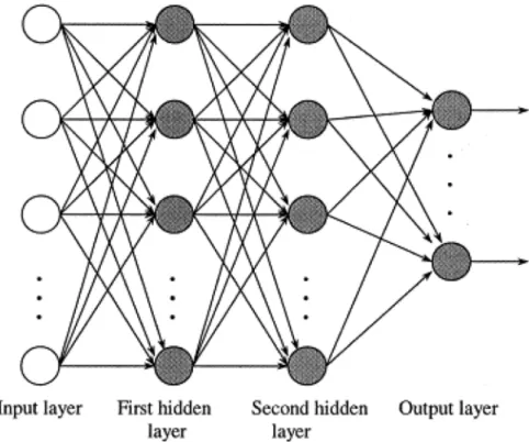
The artificial neural network learning algorithm adopted for our study of α decay of heavy nuclei is based on the feedforward multilayer perceptron architecture sketched in Fig. 1, consisting of an input layer, an output layer, and one or more intermediate (“hidden”) layers, each
composed of “nodes” or neuron-like units. Information flows exclusively from input to hidden to output layers. For simplicity, we consider here only one hidden layer, consisting a number J of nodes j that serves as a hyper-parameter. (Generalization to multiple hidden layers is straightforward). Ordinarily, every node in a given layer provides input to every node in the succeeding layer, with no reciprocal connections; in this respect the net-work is fully connected.
The input layer is composed of I nodes i that serve only as registers of the activities xi of each input pattern.
How-ever, the J nodes j of the hidden layer and the K nodes k of the output layer process, in turn, their respective inputs xi and hj in a manner typically analogous to
bio-logical neurons. This produces corresponding outputs hj = f (bj +∑i wjixi) and
(2) in terms of IJ + JK connection weights plus J + K bias parameters: collectively w = {wji, wkj} and b = {bj, bk}. For the application reported here, the activation (or “fir-ing”) function f of processing units in the middle layer fig. 1: Conventional multilayer feedforward neural network (Multilayer Perceptron) having two intermediate layers of “hidden neurons” between input and output
layers. Darkened circles represent processing units analogous to neurons; lines oriented forward symbolize weighted connections between units analogous to interneuron synapses. information flows left to right as units in each layer simulate those in the next layer.
DeCeMBeR 2019 vol. 29 no. 6 apctp sectiOn
was chosen as f (u) = tanh(u), resembling the response of biological neurons.
Here we must note that because regression is the main task to be performed in our application, the outputs are not required to lie in any particular interval. Accordingly, outputs of the network are better computed as linear combinations of the outputs of the hidden layer plus a bias. This is the same as not considering any activation function in the output layer.
The collection w of weights of the connections from input to hidden units and from the hidden units to the output units, together with the biases b of these units, determine the given MLP as a proposed solution of the regression problem represented by Eq. (1). In the backpropagation learning algorithm, the weights are commonly optimized by gradient-descent minimization of the loss function
(3) which is constructed from a sum of squares of output errors for the nt examples provided by the training set,
plus a simple regularization term that punishes weights of large magnitude. In our implementations of gradient descent, large weight oscillations are discouraged by a “classical” momentum term [20] in each training step s, according to
(4) (or alternatively with Nesterov’s momentum [21]). Here ∇Lw denotes the gradient of the loss function evaluated
at w, while 0 < α < 1 is the learning rate and 0 ≤ µ < 1 is the momentum parameter. (Also implemented in our applications are adaptive moments (“Adam”) [22], in-volving moving averages of gradient and squared gradi-ent, bias correction for second moments, and associated weight updating.) We refer the reader to the standard texts [23–25] for more thorough and authoritative intro-ductions to neural networks and machine learning. SPECIALIZATION TO MACHINE LEARNING (ML) OF ALPHA DECAY
In our exploratory study, we focus attention on one
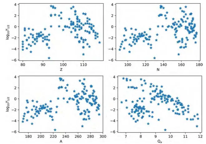
spe-fig. 2: visualizations of measured experimental alpha-decay half-lives (in log10 scale) for the 150 nuclei in the chosen database,
cific application of ML to statistical modeling and pre-diction of nuclear properties, namely α-decay lifetimes of heavy nuclei, based on the multilayer perceptron pro-cedures outlined in the preceding section. Additionally, some results of alternative strategies for exploration of the same problem domain will be summarized.
For this ML application, the data involved in both ML statistical modeling and assessment of the theoretical model chosen as reference include:
(i) The experimental half-lives Texp
1/2(measured in
sec-onds) of a set of 150 nuclear isotopes (N, Z) with Z ≥ 104.
(ii) Corresponding experimental values of the energy release Qα(Z, N), which is M(Z, N) – M(Z – 2, N – 2) – M(2, 2) in terms of reactant masses.
These data sets, assembled from Refs. [15, 16], contain entries for the 120 neutron-deficient nuclides in Table I of Ref. [16], supplemented by entries for the 30
non-overlapping nuclides with Z =80 – 118 drawn Table I of Ref. [15]. (Sources for the experimental values are cited in these two studies; such values and their uncertainties may differ from those provided by the National Nuclear Data Center.) Fig. 2 displays plots of the experimentally determined log T1/2 values versus Z, N, A, and input Qα, for the composite data set of 150 nuclides.
Inputs to the MLP network models include Z, N, their parities, and their distances dZ and dN from respective
proton and neutron magic numbers, viz. 2, 8, 20, 28, 50, 82, and 126 for Z, plus 184 for N, for a total of 7 inputs, including the experimental Qα values.
As is conventional in modeling of decay rates, the actual quantity targeted is the base-10 logarithm t = log10T1/2
of the half-life T1/2 (in seconds).For a given model of the
half-life data (whether theoretical or statistical), the key figure of merit is the smallness of the standard deviation
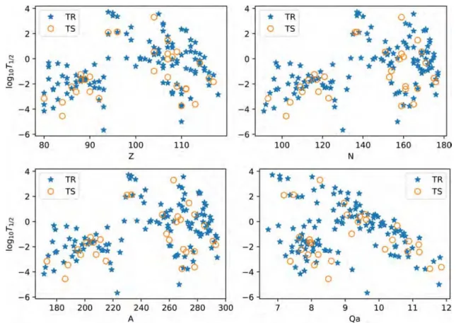
(5) fig. 3: visualizations of the training set (tR) and test set (tS) adopted for Net1, plotted with respect to atomic number Z, neutron
DeCeMBeR 2019 vol. 29 no. 6 apctp sectiOn
of the model estimates from experiment. If the ML pro-cedure is used in the alternative mode of modeling the differences between a given theoretical model (th) and ex-periment (exp), so as to develop a statistical model of the “residuals” (res), the second term within the parentheses in Eq. 5 is replaced by –tth
n – tresn .
Inputs to the neural network model, I = 7 in total, con-sist of the atomic and neutron numbers Z and N, their parities, the decay energy Qα, and the distances |Z – Zm|
and |N – Nm| of a given input nuclide from the nearest
respective magic numbers (viz. 8, 20, 28, 50, 82, 126 for protons, plus 184 for neutrons).
For model assessment, the full data set was randomly split into:
(i) A training set (TR), comprised of 80% of the data (120 nuclear “patterns”).
(ii) A test set (TS), 20% of the data (30 patterns), pro-vided by the remainder.
Model selection was carried out by five-fold cross-vali-dation, as explained in the preceding section. A total of 2750 combinations of (J, λ, α, µ) values (i.e. number of hidden units, regularization strength, learning rate, and momentum) were compared. The specific learning algo-rithm applied was gradient descent with Nesterov’s mo-mentum. The number of epochs (passages through the training data) was 3000. Batch updating (batch size = 32) was applied, with data shuffling. During the learning phase, the quality measure σ was monitored at each ep-och. Weights/biases were chosen to minimize σ(TR) over epochs. These network parameters were then used to
make predictions for new nuclear examples, outside the training set.
Two kinds of network model were constructed:
(i) Net1: Trained on the experimental half-life data for the selected 150 nuclear examples drawn from Refs. [15, 16], yielding a purely statistical model of α decay. Fig. 3 provides different visualizations of the training and test sets used for this network model.
(ii) Net2: Trained on the data set consisting of the differ-ences between the predictions of a given theoretical model of α decay (specifically, ELDM) and experi-ment, providing statistically derived corrections to this model.
After finding the best combinations (J*, λ*, α*, µ*) of hy-perparameters for Net1 and Net2, the most favored nets were trained again, but now using the whole set of train-ing data at once.
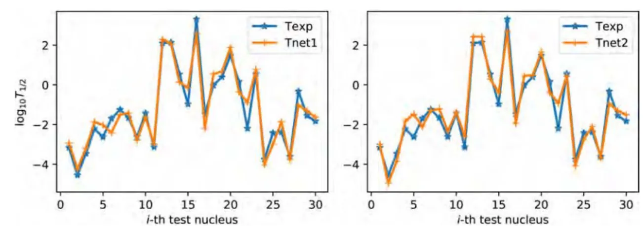
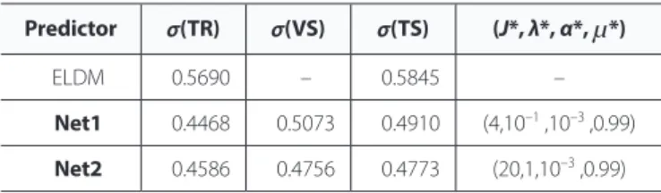
RESULTS FOR LEARNING AND PREDICTION Table 1 summarizes the results of these machine-learn-ing procedures applied to α-decay half-life data for the 150 heavy nuclei extracted from Refs. [15, 16]. Opti-mal sets of the parameters (J, λ, α, µ) are shown for the two network models, along with the respective quality measures σ attained by these nets on training, valida-tion, and test sets, respectively denoted TR, VS, and TS. Corresponding values of the standard-deviation qual-ity measure σ as achieved with the theoretical models employed by Cui et al. in these references are entered for comparison. Fig. 4 gives a schematic view of the fig. 4: Schematic representation of the performance of Net1 and Net2 in prediction of half-lives of test nuclides.
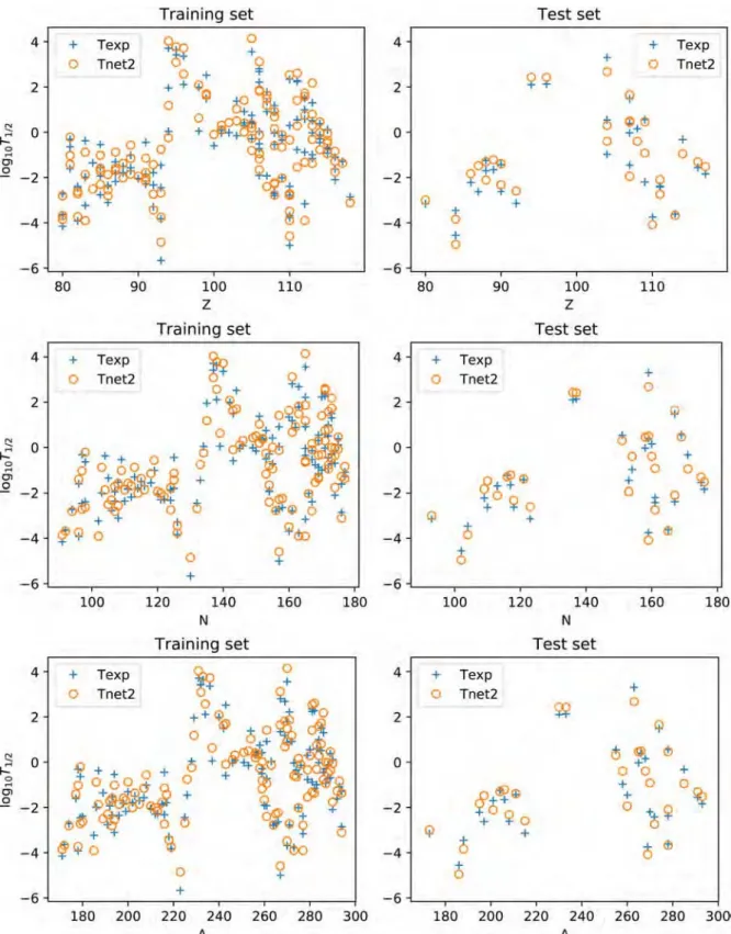
quality of prediction achieved by Net1 and Net2. Fig. 5
provides more refined graphical representations of the performance of Net2 on training and test sets.
fig. 5: ensembles of half-life fits for training nuclei and predictions for test nuclei, generated by Net2 and plotted versus atomic
DeCeMBeR 2019 vol. 29 no. 6 apctp sectiOn
table i. Summary of machine-learning results for the quality measure σ,
compared with corresponding results from the theoretical models applied in Refs. [15, 16]. Also displayed are the optimal parameter choices used for the Ml models.
predictor σ(tr) σ(vs) σ(ts) (J*, λ*, α*, µ*)
elDM 0.5690 – 0.5845 –
net1 0.4468 0.5073 0.4910 (4,10–1 ,10–3 ,0.99) net2 0.4586 0.4756 0.4773 (20,1,10–3 ,0.99)
CONCLUSIONS AND OUTLOOK
Table 1 shows a modest reduction of the error measure σ of the theoretical models upon implementing machine learning, although it is clear that ML is quantitatively competitive with the best of current quantum-mechanical models of α decay. It is significant, however, that quite unlike what is found in ML of nuclear masses [1, 2] there is no appreciable improvement relative to the perfor-mance of the purely statistical ML model provided by Net1, when machine learning is applied to create Net2 by training only on the residuals of the chosen theoreti-cal model.
There are several possible explanations for these find-ings. A major consideration is the paucity of data com-pared to the machine learning of nuclear masses. For α decay, the examples available for training are at most of order hundreds, whereas for masses there between two and three thousand measurements that may be used for training. It was for this reason that we chose to enlarge the α-decay data set of Ref. [16] by adding non-overlap-ping examples from the data set of Ref. [15]. This may have been counterproductive in that all of the added nuclei have Z > 104, whereas the data set of Ref. [16] is made up of neutron-deficient nuclei. More broadly, the irreducible sparsity of training data increases the danger of overlearning and accentuates the sacrifices made in its avoidance.
These considerations would not be so serious were it not for the fact that the experimental measurements of α and β decay rates are subject to relatively large errors compared to masses. This is responsible for the accepted rule-of-thumb that α-decay half-life predictions (mea-sured in seconds) within an order of magnitude of the true value are considered acceptable (cf. the ”hindrance factor”). The clear implication is that in ML applications to nuclear decay, the learning algorithm should give ex-plicit consideration to the noisy component of the data,
to the extent it is quantifiable. A straightforward modi-fication of the backpropagation algorithm to cope with this situation has been developed and tested in Ref. [26], and will be implemented in further ML treatments of α decay.
The otherwise unexpected results of an additional ex-periment carried out as a limiting case are relevant to the situation described. We sought to answer the ques-tion: How well does a degenerate version of the network model considered here, i.e., the Elementary Perceptron, perform on the alpha-decay problem? The answer is contained in Table 2, where Net1 and Net2 now have only a single processing layer (the output layer).
table ii. Performance of the elementary Perceptron in learning and prediction
of alpha-decay half-lives (cf. table 1). Also displayed are the optimal parameter choices used for the Ml models.
predictor σ(tr) σ(vs) σ(ts) (J*, λ*, α*, µ*)
net1 0.4840 0.5309 0.5153 (0,0,10–2 ,0.0) net2 0.4399 0.4837 0.4638 (0,0,10–2 ,0.99) These results are not inconsistent with the above discus-sion. In the context of the alpha-decay machine-learning problem where uncertainties in measured half-lives are large, coarse data can be modeled just as well by a coarse model.
Acknowledgments: JWC expresses his gratitude for the hospitality of the University of Madeira during extended residence, and continuing support from the McDonnell Center for the Space Sciences.
References
[1] J. W. Clark, S. Gazula, in Condensed Matter Theories, Vol. 6, S. Fantoni, S. Rosati, eds. (Plenum, New York, 1991), pp. 1-24; S. Gazula, J. W. Clark, H. Bohr, Nucl. Phys. A 540, 1 (1992); K. A. Gernoth, J. W. Clark, J. S. Prater, H. Bohr, Phys. Lett. B 300, 1 (1993); K. A. Gernoth, J. W. Clark, Neural Networks 8, 291 (1995); J. W. Clark, T. Lindenau, M. L. Ristig, Scientific Applications of Neural Nets (Springer, Berlin, 1999); Springer Lecture Notes in Physics, Vol. 522; J. W. Clark, K. A. Gernoth, S. Dittmar, M. L. Ristig, Phys. Rev. E 59, 6161 (1999); J. W. Clark, H. Li, Int. J. Mod. Phys. B 20, 5015 (2006), arXiv: nucl-th/0603037; S. Athanassopoulos, E. Mavrommatis, K. A. Gernoth, J. W. Clark, in Advances in Nuclear Physics, Proceedings of the 15th Hellenic Symposium on Nuclear Physics, G. A. Lalazissis, Ch. C. Moustakidis, eds. (Art of Text Publishing & Graphic Arts Co., Thessaloniki, 2006), pp. 65-70, arXiv: nucl-th/0511088; N. Costiris, E. Mavrommatis, K. A. Gernoth, J. W. Clark, Phys. Rev. C 80, 044332 (2009), arXiv:nucl-th/0806.2850; N. J. Costiris, E. Mavrommatis, K. A. Gernoth, J. W. Clark, arXiv:nucl-th/1309.0540; S. Akkoyun, T. Bayram, S. O. Kara,
A. Sinan, J. Phys. G: Nucl. Part. Phys. 40, 055106 (2013); T. Bayram, S. Akkoyun, S. O. Kara, Ann. Rev. Nucl. Energy 63, 172 (2014); T. Bayram, S. Akkoyun, S. O. Kara, Journal of Physics: Conference Series 490, 012105 (2014).
[2] R.Utama, J.Piekarewicz, H. B. Prosper, Phys.Rev.C 93, 1 (2016); R. Utama, J. Piekarewicz, Phys. Rev. C 97, 1 (2018).
[3] H.F. Zhang, L. H.Wang, J. P. Yin, P. H.Chen, H. F. Zhang, J. Phys. G:Nucl. Part. Phys. 44, 045110 (2017).
[4] G.A. Negoita, J. P.Vary, G. R. Luecke, P.Maris, A. M.Shirokov, I. J. Shin, Y. Kim, E. G. Ng, C. Yang, M. Lockner, G. M. Prabhu, Phys. Rev. C 99, 054308 (2019). [5] L. Neufcourt, Y. Cao, W. Nazarewicz, F. Viens, Phys. Rev. C 98, 1 (2018),
arXiv:1806.00552.
[6] Z. M. Niu, H. Z. Liang, B. H. Sun, W. H. Long, Y. F. Niu, Phys. Rev. C 99, 064307 (2019).
[7] J. H. Hamilton, S. Hofmann, Y. T. Organessian, Ann. Rev. Nucl. Part. Sci. 63, 383 (2013).
[8] V. E. Viola, G. T. Seaborg, J. Inorg. Nucl. Chem. 28, 741 (1966). [9] G. Royer, Nucl. Phys. A 848, 279 (2010).
[10] V. Yu. Denisov, A. A. Khkudenko, Phys. Rev. C 79 054614 (2009); 82, 059901(E) (2010).
[11] G. Royer, B. Remaud, J. Phys. G: Nucl. Part. Phys. 8,
[12] J. P. Cui, Y. L. Zhang, S. Zhang, Y. Z. Wang, Int. J. Mod. Phys. E 25, 1650056 (2016).
[13] M. Goncalves, S. B. Duarte, Phys. Rev. C 48, 2409 (1993).
[14] S. B. Duarte, O. Rodriguez, O. A. P. Tavares, et al., Phys. Rev. C 57, 2516 (1998).
[15] J. P. Cui, Y. L. Zhang, S. Zhang, Y. Z. Wang, Phys. Rev. C 97, 014316 (2018). [16] J. P. Cui, Y. Xiao, Y. H. Gao, Y. Z. Wang, Nucl. Phys. A 987, 99 (2019). [17] K. P. Santhosh, C. Nithya, H. Hassanabadi, D. T. Akrawy, Phys. Rev. C 98,
024625 (2018).
[18] T. Bayram, S. Akkoyun, S. O. Kara, Journal of Physics: Conference Series 490, 012105 (2014).
[19] U. B. Rodriguez, C. Z. Vargas, M. Goncalves, S. Barbosa Duarte, Fernando Guzman, J. Phys. G: Nucl. Part. Phys. 46, 115 (2019).
[20] N. Qiang, Neural Networks 12, 145 (1999).
[21] Y. Nesterov, Soviet Mathematics Doklady 27, 372 (1983). [22] D. P. Kingma, J. Ba, Adam: A method for stochastic optimization,
International Conference on Learning Representations 2015, pp. 1-13, arXiv:1412.6980.
[23] S. Haykin, Neural Networks and Learning Machines (Prentice Hall, New York, NY 2008).
[24] C. M. Bishop, Neural Networks for Pattern Recognition (Oxford University Press, Birmingham, UK, 1995).
[25] R. M. Neal, Bayesian Learning for Neural Networks, Lecture Notes in Statistics, Vol. 118 (Springer, New York, NY, 1996).