Integrating Protein Structural Information

(1)

Ludwig Krippahl

Integrating Protein Structural Information

Dissertação apresentada para obtenção de Grau de Doutor em Bioquímica, Bioquímica Estrutural, pela Universidade Nova de Lisboa, Faculdade de Ciências e Tecnologia.

(2)

(3)

(4)

(5)

Acknowledgements

Anytime you see a turtle up on top of a fence post, you know he had some help.

Alex Haley, paraphrased.

My work on molecular modelling began eight years ago, as a naïve undergraduate student of a bioinorganics course, when I proposed to write a protein docking program instead of the course’s regular assignment, which was a simple experimental protocol. Fortunately, the course lecturer was both generous and understanding, and let me off with a much simpler task. Little did I know that eight years later I would still be working with Professor José Moura on the assignment I had initially proposed. What I achieved these seven years I owe to the chance he gave me and to his constant support, orientation, and friendship.

It was also at that time that I began working with Doctor Nuno Palma, and most of my work on BiGGER and Chemera was under his supervision. We worked extraordinarily well together, and our complementary views on most problems led me much farther than I could ever have gone otherwise. Working with Doctor Palma was a wonderful experience, and I could not have developed the docking algorithms without his supervision, his knowledge of molecular modelling, and his skill at finding the right tests and test cases to show us the problems along the way.

Professor Pedro Barahona was the lecturer on the constraint programming course in the artificial intelligence master programme. Both the subject and the way it was presented aroused my interest in constraint programming, and led me to the application of these techniques to protein structure and interaction. The PSICO algorithm was developed under the guidance, and with the teachings, of Professor Barahona, and much of the credit should go to his orientation, experience, and interest in the problem of determining protein structures.

(6)

iv

(7)

Sumário

O tema principal deste trabalho é a aplicação de técnicas de programação por restrições e outras técnicas de inteligência artificial à modelação de estrutura e interacção de proteínas, com o objectivo de melhor combinar dados experimentais com métodos de previsão estrutural.

A primeira parte desta dissertação introduz os temas principais de estrutura de proteínas e programação por restrições, resume as técnicas mais recentes de modelação de estruturas e complexos de proteínas, descreve o contexto em que se inserem as técnicas descritas nas partes subsequentes, e delineia o ponto fulcral da tese: a integração de dados experimentais na modelação.

O primeiro capitulo, Protein Structure, introduz o leitor às noções básicas de estrutura de amino ácidos, cadeias proteicas, e enrolamento e interacção de proteínas. Estes são conceitos importantes para compreender o trabalho descrito nas partes dois e três..

O segundo capitulo, Protein Modelling, dá uma visão breve das técnicas experimentais e de previsão teórica usadas para criar modelos de estruturas proteicas. Este capítulo dá o contexto onde se insere o trabalho descrito nas partes dois e três, mas não é essencial para a compreensão dos algoritmos apresentados.

O terceiro capítulo, Constraint Programming, delineia os conceitos principais desta técnica de programação. A compreensão de métodos de modelação de variáveis, noção de consistência e programação, e de métodos de pesquisa ajudará o leitor interessado nos detalhes dos algoritmos descritos na segunda parte desta dissertação.

O quarto capítulo, Integrating Structural Information, resume a tese aqui proposta, os objectivos deste trabalho, e dá uma ideia de como os algoritmos desenvolvidos podem contribuir para a modelação de estruturas de proteínas. O objective principal é obter um sistema flexível e em evolução continua para a integração de dados experimentais e previsões teóricas.

(8)

vi

O capitulo cinco, The PSICO Algorithm, descreve as componentes principais deste agoritmo para previsão e determinação de estruturas de proteínas. Estas incluem a modelação de domínios e variáveis, restrições binárias de distância, restrições sobre grupos rígidos e ângulos de torção, e detecção de sobreposições de átomos. Este capitulo descreve também como os diferentes métodos de propagação são integrados e as heurísticas usadas para guiar a pesquisa de soluções.

O sexto capitulo, The BiGGER Algorithm, descreve o algoritmo de modelação de complexos de proteínas. Detalha o filtro geométrico e a pesquisa geométrica de modelos candidatos, e o algoritmo de avaliação que estima a viabilidade destes modelos. O capitulo seis descreve também a integração de restrições experimentais na fase de pesquisa e eliminação, usando técnicas de programação por restrições..

O capítulo sete, Algorithms in Chemera, descreve um conjunto de algoritmos auxiliares para visualizar estruturas e propriedades de proteínas. Alguns dos algoritmos apresentados neste capítulo tais como os de agrupamento ou avaliação de simetria de complexos são um complemento ao algoritmo BiGGER, permitindo um processamento adicional dos modelos gerados pelo algoritmo de previsão de complexos.

A terceira parte desta dissertação apresenta os resultados experimentais usados para testar e parameterizar os algoritmos, bem como exemplos de aplicações práticas a casos reais, e é parte da contribuição original deste trabalho.

O capítulo oito foca os testes do algoritmo PSICO, usando principalmente dados simulados. Este capítulo delineia também alguns problemas que só poderão ser adequadamente resolvidos quando o algoritmo começar a ser aplicado a casos reais.

O capítulo nove descreve a parameterização da fase de pesquisa e triagem geométrica do algoritmo BiGGER, bem como o trabalho mais recente no aperfeiçoamento das funções de avaliação dos modelos gerados.

(9)

deste algoritmo a problemas gerais de escala multi-dimensional (Multidimensional Scaling), que usam parte dos mecanismos de propagação e pesquisa do algoritmo PSICO para produzir valores iniciais para algoritmos de optimização por pesquisa local.

(10)

(11)

Abstract

The central theme of this work is the application of constraint programming and other artificial intelligence techniques to protein structure problems, with the goal of better combining experimental data with structure prediction methods.

Part one of the dissertation introduces the main subjects of protein structure and constraint programming, summarises the state of the art in the modelling of protein structures and complexes, sets the context for the techniques described later on, and outlines the main points of the thesis: the integration of experimental data in modelling.

The first chapter, Protein Structure, introduces the reader to the basic notions of amino acid structure, protein chains, and protein folding and interaction. These are important concepts to understand the work described in parts two and three.

Chapter two, Protein Modelling, gives a brief overview of experimental and theoretical techniques to model protein structures. The information in this chapter provides the context of the investigations described in parts two and three, but is not essential to understanding the methods developed.

Chapter three, Constraint Programming, outlines the main concepts of this programming technique. Understanding variable modelling, the notions of consistency and propagation, and search methods should greatly help the reader interested in the details of the algorithms, as described in part two of this book.

The fourth chapter, Integrating Structural Information, is a summary of the thesis proposed here. This chapter is an overview of the objectives of this work, and gives an idea of how the algorithms developed here could help in modelling protein structures. The main goal is to provide a flexible and continuously evolving framework for the integration of structural information from a diversity of experimental techniques and theoretical predictions.

(12)

x

Chapter five, The PSICO Algorithm, describes the main components of this algorithm for predicting and determining protein structure. These include the modelling of the variable domains, binary distance constraints, n-ary group constraints, torsion angle constraints and global atom overlap inconsistency detection. The chapter also describes how the different propagation methods are integrated, and the heuristics used to guide the search for a solution.

Chapter six, The BiGGER Algorithm, describes the algorithm for modelling protein interactions. It details the geometric search and filtering of likely candidates, and the scoring algorithms to estimate the likelihood of each retained model being an accurate representation of the real complex. Chapter six also describes the integrating experimental data in the search stage of the algorithm, using constraint programming techniques.

Chapter seven, Algorithms in Chemera, describes a set of auxiliary algorithms for the visualisation of protein structures and properties. Some of these algorithms, such as clustering, symmetry score evaluations and scoring of docking constraints are a complement to the BiGGER algorithm, serving to further process the models generated by the docking algorithm.

The third part of this dissertation presents the experiments and results that validate the methods, and describes their application. It is part of the original contribution of this work, describing the experiments to test and parameterize the algorithms, and the practical applications of these algorithms.

Chapter eight focuses on the testing of PSICO, using mostly simulated data. This chapter also outlines several issues with this algorithm that can only be properly resolved using experimental data, something not yet done at this stage.

Chapter nine addresses the parameterization of the geometric search and filtering stages of the BiGGER algorithm, and the more recent and ongoing work on the scoring functions that evaluate the candidate models.

(13)

Multidimensional Scaling, which uses part of the PSICO propagation and search mechanisms to provide initial values for dissimilarity searches in this field.

(14)

xii

10.2 Electron Transfer between Aldehyde Oxydoreductase and Flavodoxin 114 10.3 Electron Transfer Complexes between Cytochrome c550 and Cytochrome c Peroxidase 118 10.4 Electron Transfer Complex between Cytochrome c553 and Ferredoxin 120 10.5 Electron Transfer Complex between Ferredoxin and Ferredoxin NADP+ Reductase 121 10.6 Electron Transfer Complex between Cytochrome b5 and Cytochrome C 123

10.7 The CAPRI Experiments 123

10.8 Combining PSICO with Multidimensional Scaling 129

11 Concluding Remarks 135

References 137

APPENDIXES 145

Appendix I: PSICO Dynamic Link Library 147

AI. 1. Initialisation, Finalisation, and Problem Selection functions 147

AI. 2. Atom Handling Functions 148

AI. 3. Enumeration and Backtracking Functions 149

AI. 4. Propagation and Domain Handling Functions 150

AI. 5. Group Handling Functions 150

AI. 6. Optimisation Functions 151

AI. 7. Debugging Functions 151

AI. 8. Other Functions 151

Appendix II: Tables 153

Glossary 158

(16)

xiv

Table of Figures

Figure 1-1 A short segment of four amino acids. The backbone is outlined in gray, and the atoms are represented in different colours (nitrogen in blue, carbon in white, oxygen in grey, hydrogen atoms are not shown). The backbone atoms are outlined in grey, with each N-C-C sequence belonging to one amino acid (from top to bottom). Each amino acid has a unique side chain... 4 Figure 1-2 Example of two domains in the desufloferrodoxin monomer (Coelho and others 1997), in

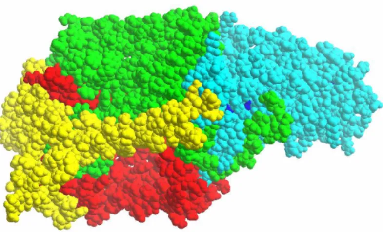
dark blue and in orange. Different domains are not only distinct structural motifs, but can also have different and independent functions. ... 6 Figure 1-3 The structure of the photosynthetic reaction center from Rhodopseudomonas viridis

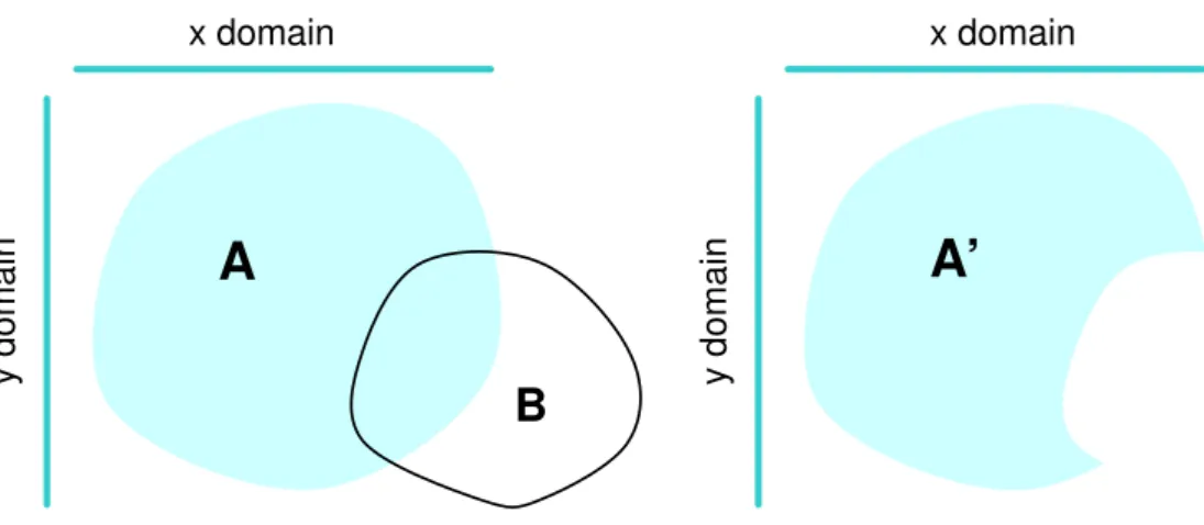
(Deisenhofer and otherrs 1984). Different protein monomers are shown in different colors. The whole protein consists of four different protein sub-units plus a large number of non-protein co-factors. ... 7 Figure 5-1 Excluding atom A from region X requires a simple alteration in the domain of A if the

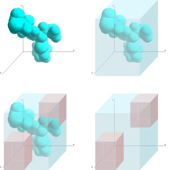
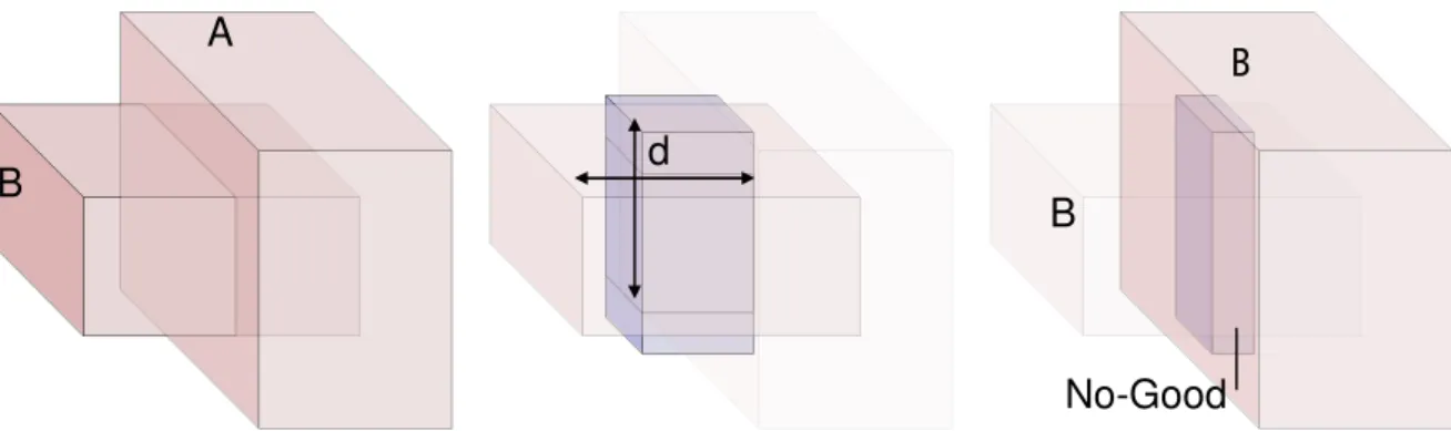
coordinates of A are modelled together, but the separate x and y domains, represented by the bars, are not changed by removing the region X from domain A... 29 Figure 5-2 The domain of an atom (top left) is represented using a simple cuboid block (top right),

the Good region, plus A set of zero or more additional blocks represents the no-Good region, from which the atom is excluded (bottom). ... 30 Figure 5-3 Modelling distance constraints as cubic regions. On the left a sphere defined by the

Euclidean distance to a point- On the centre, the cube modelling an In Constraint, with an edge of twice the distance value. On the right, the cube modelling an Out Constraint, with an edge of twice the distance value divided by the square root of three... 32 Figure 5-4 Propagation of an In Constraint. The left panel shows the Good Regions of the two atom

domains. The centre panel shows the neighbourhood region of atom B, and the right panel shows the new domain of atom A, which was restricted to the intersection with the neighbourhood of the atom B. ... 33 Figure 5-5 Propagating the Out Constraint. The left panel shows the Good Regions of two

overlapping domains. The central panel shows the exclusion region of atom B. The right panel shows the intersection of the exclusion region with the good region of atom A, which is added to the No-Good Regions of atom A... 34 Figure 5-6 The three atoms A, B, and C, form a rigid group (dark orange circles), and each atom is

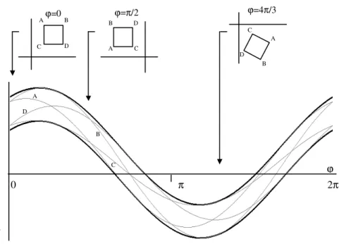
restricted to a rectangular domain. The left panel shows the limits for a horizontal translation, and the right panel shows the limits for a vertical translation (light orange circles with dashed line). The dashed boxes on the right panel indicate the accessible regions for each atom with the group in this orientation. ... 36 Figure 5-7 The position of an atom relative to the center of the group as a function of the rotation

angle ψ can be expressed as a sine function with amplitude A and phase α’. The position of the center relative to the atom is a similar curve, but with the phase shifted by 180º (α), giving the sine line shown on the right... 37 Figure 5-8 Each atom constrains the translation of the group as a function of the domain of the

(17)

the two atom positions are compatible and the corresponding constraints on the translation of the whole group in this orientation... 38 Figure 5-9 The thick lines show the lines obtained by adding δ (top line) and subtracting δ (bottom

line) to the line defined by the centre of the coordinates interval. The top panels show three orientations of the rectangle defined by the coordinate intervals. A, B, C, and D are the extreme points of the rectangle, and thin lines in the lower diagram show their trajectories as a function of the ϕ rotation parameter. ... 42 Figure 5-10 Two rigid groups, A and B, joined by a rotatable bond (1). Note that the two atoms on

both ends of bond 1 belong to both groups, since rotation around this axis does not change the position of these atoms relative to the atoms in A or B. There are other bonds and other groups in the figure, but not all are displayed, for clarity. Atoms are coloured by element: C white, N blue, O red. Hydrogen atoms are not displayed... 44 Figure 5-11 Calculating the minimum volume occupied by B (domain shown as a dashed box) in the

domain of A. Atom B is considered to be as far as possible from A (white circle), and occupies the region shown in orange. The red box shows the minimum volume B occupies in A. ... 45 Figure 5-12 Evolution of the enumeration cycle. From left to right, after one iteration, 15, 30 and

300. The last panel shows only the backbone for clarity... 49 Figure 5-13 The torsion angle model. The panel on the left shows the data structure as a tree, with

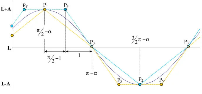
atom groups for nodes and dihedral angles for arcs. The panel on the left shows the respective protein structure... 50 Figure 5-14 Piecewise linear upper and lower bounds (blue and orange, respectively) for a sine line.

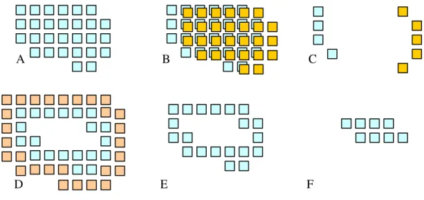
See text for how to calculate the points... 54 Figure 6-1 Using Boolean operations to determine the surface and core regions. Panel A shows the

initial grid. A copy of this grid is shifted one cell to the right (B) and combined with the original using an XOR operation (C). Panel D shows the total (using OR operation) of all XOR combinations. Panel E shows the trimmed surface grid, and F the core grid. Filled squares represent grid cells with a value of one. ... 61 Figure 6-2 The surface and core grids (blue and orange, respectively) for the HIV protease structure

(Wlodawer and others 1989). The three panels show sections of the grid in three orthogonal planes... 61 Figure 6-3 Converting a binary grid into a segment array. The binary grid represented by blue

squares blue and dashed squares (one and zero, respectively) is converted into an array of segment lists. The fourth segment list contains two segments, (1,2) and (4,6), to represent the two disjoint segments on the fourth line of the grid. ... 62 Figure 6-4 Difference in the grids when using hard (left panel) or soft docking (right panel). Grey

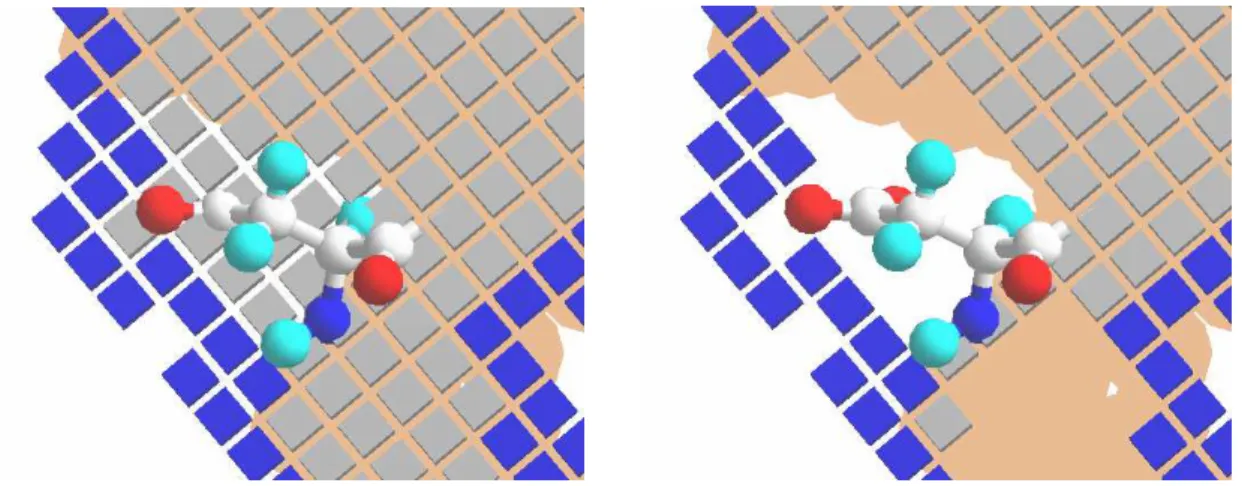
cubes represent the core grids, blue cubes the surface grids. Note that the surface grids are identical, but the core grid in the soft docking option is empty in all cells spanned by the side chain of the aspartate shown in the centre of each panel... 63 Figure 6-5 Generating the displacement domain in one dimension. The left panel shows the

(18)

xvi

the entry and exit points on the displacement array. Step three runs through the displacement array from left to right, adding the value on each cell to the value on the accumulator. The region where both atoms respect the distance constraint is shown in green... 67 Figure 6-7 Calculating the minimum overlap, for the surface contact score. The probe grids (core in

grey, surface in light blue) and the target grids (core in grey, surface in dark blue). The vertical alignment represents a given displacement value for the vertical axis. The surface cell totals for the surface grids are in the two columns of numbers adjacent to the grids. The rightmost column shows the minimum value for each row. The total of 11 means that no model obtained by searching the horizontal displacement can have an overlap score greater than 11 for this vertical displacement. ... 68 Figure 7-1 Desulforedoxin (orange) fitted to the desulforedoxin-like domain in desulfoferrodoxin

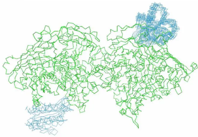
(blue). Side chains are shown as thin lines, and the backbone as thick lines. The structures used were 1DXG (Archer and others 1995) and 1DFX (Coelho and others 1996, 1997). ... 72 Figure 7-2 Two clusters of models for the docking simulation of Aldehyde Oxidoreductase (Rebelo

and others 2001), in green, complexed with an homology model for flavodoxin. ... 73 Figure 7-3 High and low symmetry complexes (left and right panels, respectively), from a docking

simulation to reconstruct the desulfoferrodoxin dimer (PDB code 1DFX). Each monomer is shown in a different color. ... 75 Figure 7-4 Three representations of the electrostatic properties of cytochrome C-522. The left panel

shows the individual atomic charges (red for negative, blue for positive), the central panel shows the total charges for each amino acid residue, and the right panel shows the dipole moment vector of this protein... 76 Figure 7-5 Shows three representations of the electrostatic field surrounding the cytochrome C552

monomer from Pseudomonas nautical. The left panel shows the field in a plane, with the colour indicating the intensity of the field (red for negative, blue for positive). The centre panel shows isopotential lines at ±0.1Kcal/mol (solid) and ±0.01Kcal/mol (dotted). The right panel shows a three-dimensional representation of the ±0.1 Kcal/mol isopotential surfaces... 79 Figure 7-6 Electron tunnelling within and between two dimers of desulfoferrodoxin (Coelho and

others 1996, 1997). The red colour indicates the probability of electron transfer from the iron atom at centre A, suggesting a possible pathway from atom A through B and to C... 80 Figure 8-1 RMSD from the target structure and computation times for the 183 test structures.

Computation times are scaled to a 1GHz PC. The red and green circles indicate the structures shown on Figure 8-2. See Table 2, page 150. ... 84 Figure 8-2 Two structures illustrating the performance of binary distance constraint propagation in

PSICO. The left panel shows the target structure (in blue) for a DNA binding protein, PDB code 1FJL (Wilson and others 1995) and the PSICO model in red. The right panel shows the target structure of a 1,3-Beta-Glucanase (Varghese and others 1994), PDB code 1GHS, in blue and the PSICO model in red. ... 85 Figure 8-3 Propagation times and final domain volumes for arc-consistency in binary distance

constraints and group propagation for a randomly generated group. Times are in seconds for a PII at 300Mz running Windows. Volumes are arbitrary units. ... 86 Figure 8-4 Propagation times and final domain volumes for arc-consistency in binary distance

(19)

Figure 8-5.Percentage of detected failures as a function of the maximum displacements of the atom coordinates. The figure shows three different group sizes (5, 10, and 20), comparing the binary arc-consistency algorithm implemented in PSICO with the group propagation described here... 89 Figure 8-6 PSICO model for desulforedoxin using experimental NOESY data (Goodfellow and others

1998), shown in red, compared with the crystallographic structure of desulforedoxin, in blue (PDB code 1DXG, Archer and others 1995). ... 90 Figure 9-1 Ranking of the highest scoring model with less than 4Å deviation from the target

complex for the 20 complexes in the test set. ... 98 Figure 9-2 Shows monomers D (red) and F(green) of Bovine F1-ATPase (PDB code 1BMF). The

remainder of the protein is shown in grey. It is more likely that the placement of these two monomers is determined by interactions with other chains in the protein than by a mutual affinity... 100 Figure 9-3 Shows the variation in the fraction of interfaces modelled with success as a function of

the added radius parameter, both with and without hydrogen atoms. An interface was successfully modelled if there was at least one model at less than 3Å RMSD from the known structure within the 10 highest scoring models. Only the surface contact score was used in this test, and the chains were placed in the correct relative orientation. ... 103 Figure 9-4 The left panel shows the percentage of complexes with at least one accurate model in

the highest scoring 30 models for a single orientation, as a function of the rotation angle of one partner rotated. The right panel shows the estimated probability of finding an accurate model for each angular step value. Note that there are three different criteria for an accurate model: 3 Å, 4Å, and 5Å... 105 Figure 9-5 Effect of the angular step on the probability of finding and retaining at least one correct

model. See equation (9.3). ... 106 Figure 9-6 Shows the average t values for the differences between the average contacts of correct

and incorrect complexes, for the three different contact vector dimensions and as a function of the contact radius modifier. The green circle shows the selected parameters (V28, with +1Å of contact radius modifier). The yellow circle shows the parameters for the previous version of the filter, using V15 and approximately +1Å of contact radius modifier. See Table 8 on page 153... 110 Figure 10-1 The electrostatic field profile of MOP at 0M and 0.5M ionic strength. Dotted lines

indicate negative potentials, full lines positive potentials. The isopotential lines are drawn at 1 and 0.1 Kcal/mol for the 0M ionic strength, and at 0.1, 0.01, and 0.001 Kcal/mol for 0.5M ionic strength. The Fe2S2 cluster is shown at the centre of each figure... 116 Figure 10-2A comparison of the three flavodoxin-MOP dockings. For each case the best ten models

(according to the electrostatic score) are represented by the FMN residue relative to the MOP monomer... 117 Figure 10-3 Comparison of the relative positions of the prosthetic groups for CO Dehydrogenase,

Xanthine Oxidase and the best model for the MOP-Flavodoxin complex. The FMN group of flavodoxin is shown at the bottom, aligned with the FAD groups of CO Dehydrogenase and Xanthine Oxidase. The Fe2S2 clusters are shown at the center of each protein... 118 Figure 10-4 Families of docking models for cytochrome c550 and cytochrome c peroxidase. One

(20)

xviii

two hemes on the peroxidase monomer are indicated by the letters E (electron transfer heme) and P (peroxidatic heme), and their atoms shown in purple. The highlighted family of solutions near the electron transfer heme contains several likely models for an electron transfer complex. Figure adapted from Pettigrew, Pauleta and others 2003. ... 119 Figure 10-5 The top row shows the positions of cytochrome c553 in the best models (circles)

relative to ferredoxin (shown in a backbone representation). The bottom row shows the same models but displaying the backbone of cytochrome c553 and the position of the ferredoxin as coloured circles. Red circles indicate a higher score, and columns A and B represent the best 1000 models according to the global score (column A) and the contact score from NMR data (column B). Column C shows the best models according to each score, and shows in red those models that score highest in both... 120 Figure 10-6 The highest scoring solutions for the Synechocystis FNR-Fd complex, using three

different scores. From left to right: NMR titration data (blue), site-directed mutagenesis data (green), and electron transfer (red). ... 122 Figure 10-7 The two models for the Synechocystis FNR-Fd complex. The ferredoxin is shown in blue,

on top, and the FNR in green. ... 123 Figure 10-8 Summary of the results for all CAPRI participants. The histograms represent all models

submitted, evaluated by the fraction of correct residues at the interface. The red bars indicate the best models of the group with the lowest average, the green bars the best models of the group with the highest average, and the blue bars the best BiGGER models. ... 125 Figure 10-9 Models for target 4 (left panel) and target 5 (right panel). The backbone of the

crystallographic structure is shown in thick lines and the backbone of the docking models in thin lines. The largest partner, on the left on each panel, is in the same position for all models. ... 127 Figure 10-10 Models for target 6 (left panel) and target 7 (right panel). The backbone of the

crystallographic structure is shown in thick lines and the backbone of the docking models in thin lines. The largest partner, on the left on each panel, is in the same position for all models. Note that the probe molecule for CAPRI target 7 was truncated before docking, and the docking models show only the fragment used for docking. ... 128 Figure 10-11 Desulforedoxin Monomer (Archer and others 1995). 260 Atoms, 5951 Constraint

pairs. The RMSD from the crystallographic structure was 2.1Å for PSICO and 0.02 Å for MDS. The average constraint violations were, respectively, 0.82 Å and 0.04 Å ... 132 Figure 10-12 Trypsin Inhibitor 448 Atoms, 11613 Constraint pairs. The RMSD from the

crystallographic structure was 2.8Å for PSICO and 0.02 Å for MDS. The average constraint violations were, respectively, 0.73 Å and 0.05 Å ... 132 Figure 10-13 Mutant P53 Anti-Oncogene (McCoy and others 1997): 514 Atoms, 12938 Constraint

pairs. The RMSD from the crystallographic structure was 2.5Å for PSICO and 0.02 Å for MDS. The average constraint violations were, respectively, 0.68 Å and 0.05 Å ... 132 Figure 10-14 Phosphotransferase (Jia and others 1993): 639 Atoms, 17206 Constraint pairs. The

RMSD from the crystallographic structure was 2.8Å for PSICO and 0.02 Å for MDS. The average constraint violations were, respectively, 0.67 Å and 0.01 Å ... 133 Figure 10-15 Barstar Mutant (Buckle and others 1994) 693 Atoms, 18996 Constraint pairs. The

(21)

(22)

(23)

Introduction

P

P AA RR TT

1

In This Part: Chapter 1

Protein Structure Chapter 2

Protein Modelling Chapter 3

Constraint Programming Chapter 4

(24)

2 Introduction

(25)

Protein Structure 3

1 Protein Structure

One unmoving that is swifter than Mind, That the Gods reach not, for It progresses ever in front. That, standing, passes beyond others as they run. (…) That moves and That moves not; That is far and the same is near; That is within all this and That also is outside all this.

Isha Upanishad, 4-5, translated by Sri Aurobindo, in "Arya" August 1914.

There are proteins in all living beings. They mediate all life processes, from growth to thought. They catalyse chemical reactions and are involved in the movements of our muscles and in the structure of our bodies. There are proteins in and around all organisms and everywhere there is life. The writers of the Vedas were unaware of this, having written the Upanishads some five thousand years ago, but even though they meant something else, theirs is an uncanny description of the role and importance of proteins.

Proteins have fascinated chemists for centuries, for solidifying when heated, unlike other substances. In 1777, Pierre Maquer called them albuminous substances, from albumin (egg white, rich in protein) with which they shared this property. Gerardus Mulder coined the term “protein”, in 1839, when he proposed that all these substances were apparently multimers of a molecule with the chemical formula of C₄₀₀H₆₂₀N₁₀₀O₁₂₀ (Mulder 1839). He was wrong in his determination of the basic molecule that formed the albuminous substances, but the name was accepted.

This chapter outlines the chemical composition and structural features of proteins. It focuses mainly on aspects important for the work presented in this book and provides only a basic description, so the author recommends additional sources, such as (Darby and Creighton 1993; Branden and Tooze 1999) for an introduction to protein structure.

1.1 Amino Acids and Primary Structure

(26)

4 Introduction

4

Figure 1-1 shows a segment of an amino acid chain. The repeating sequence of Nitrogen, Carbon, Carbon atoms is the backbone, or main chain. Branching out from the main chain we can see the amino acid side chains, which are unique to each amino acid.

Figure 1-1 A short segment of four amino acid residues. The backbone is outlined in gray, and the atoms are represented in different colours (nitrogen in blue, carbon in white, oxygen in red, hydrogen atoms are not shown). The backbone atoms are outlined in grey, with each N-C-C sequence belonging to one amino acid residue (from top to bottom). Each amino acid residue has a unique side chain.

The amino acid side chains have important properties that affect both the structure and the function of the protein. Their interaction with solvent is one example. The interaction of some side chain groups with water molecules is as favourable as the interaction between water molecules, or even more favourable, and this makes the side chains hydrophilic. For other amino acids, the interaction with the water molecules is not as favourable, suffering an entropy penalisation for forcing the surrounding water molecules to reorganise.

Charge distribution is another important factor, as electrostatic attraction and repulsion is often crucial for complex formation, not only to keep the proteins together, but also to guide them to the correct configuration. It is also important in the folding of the protein, though not as important as hydrophobicity or hydrogen bonding for this. Hydrogen bonding, the sharing between two atoms of a loosely bonded hydrogen atom, is the last major factor for protein folding and complex formation. It stabilizes the main motifs of protein structure, and effectively binds proteins together in protein complexes.

Tyrosine Leucine

(27)

Protein Structure 5

1.2 Secondary Structure

Protein chains form several characteristic local structures due to hydrogen bonds between main chain atoms of different amino acids. The peptide bond between two amino acid residues locks the carboxylic oxygen and C' carbon of one residue and the amidic nitrogen and hydrogen of the other in a plane, and does not allow these atoms to rotate out of the plane. However, the bonds linking the alpha carbon to the C' Carbon and the main chain Nitrogen allow for a range of rotations. The angles of rotation around these bonds, known as phi and psi, respectively, determine the secondary structure and, ultimately, the folding of the protein.

One example is the alpha-helix, in which the main chain forms a spiral, with the phi and psi angles ranging from -60º to -50º. The alpha helix has 3.6 amino acids per turn, and hydrogen bonds between the oxygen of one residue n and the nitrogen of residue n+4 gives it great stability. Less common variants are the pi helix, in which the hydrogen bonds are formed between n and n+5, or the 310 helix, with hydrogen bonds to residue n+3.

Another important example is the beta strand. This local structure consists of usually 5 to 10 residues in a fully extended configuration (phi and psi angles close to 180º). Beta strands can bind together to form beta sheets, also stabilized by hydrogen bonds between the hydrogen of the amino groups and the oxygen of the carboxyl groups.

Secondary structures can combine to form structural motifs, or supersecondary structures. These are very important for structural modelling for several reasons. One reason is predictability; from sequence data alone it is possible to predict secondary structures and motifs with a 70% accuracy (Frishman and Argos 1997; Baldi and Brunak 1998; Wang and others 1999). Another reason is the conservation of secondary structure within protein families, both because of its strong correlation with local amino acid sequences and because evolution seems to favour the conservation of local structures in general (for example, Gille and others 2000). Finally, secondary structure elements are often easier to identify from experimental data, which even allows automated assignment procedures in multidimensional NMR spectroscopy (Bailey-Kellogg and others 2000).

1.3 Folding

(28)

6 Introduction

6

protein interacts with other molecules. Knowing the tertiary structure is crucial for understanding and manipulating the reaction pathways in living organisms.

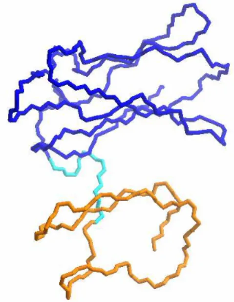
Often, a protein chain forms regions with separate hydrophobic cores. These regions are called domains, and can operate independently, as if they were several different proteins kept together by peptide linkers. Figure 1-2 shows two domains of desulfoferrodoxin.

Figure 1-2 Example of two domains in the desufloferrodoxin monomer (Coelho and others 1997), in dark blue and in orange. Different domains are not only distinct structural motifs, but can also have different and independent functions.

The semi-independence of protein domains makes these structural features the natural unit of protein structure and function. When comparing different proteins, or even protein systems, it is often necessary to take into account the modular nature of protein chains.

1.4 Protein Interactions

Most, if not all, proteins interact with other proteins. These interactions range from transient contacts, in which the partners meet briefly to perform some chemical reaction, to life-long partnerships, with each protein chain specifically adapted to be permanently associated to its partners. The structure of such assemblies of protein chains is the quaternary structure.

(29)

Protein Structure 7

(30)

8 Introduction

8

2 Protein Modelling

There's a reason physicists are so successful with what they do, and that is they study the hydrogen atom and the helium ion and then they stop.

Richard Feynman

Quantum mechanics is a powerful tool to understand the dynamics of sub-atomic particles and simple atoms and molecules. However, our capacity to analyse the details of molecular systems decreases as complexity increases, and proteins are perhaps the most complex molecules known. Though smaller than DNA and some other polymers, their versatility and the diverse roles they play in chemical reactions make it very hard to predict and model all their features in detail.

This chapter focuses on the modelling of one aspect of proteins: their structure. By protein structure one usually means an average three-dimensional configuration of the atoms in the protein, sometimes with a cursory indication of the mobility of each part of the protein chain. There are other important aspects, from folding to function, which are the subjects of much research, but fall outside the scope of this work. After an historical overview of protein structure modelling, this chapter addresses the most important experimental techniques for determining protein structures, and some prediction methods currently available. The emphasis is on Nuclear Magnetic Resonance (NMR) techniques and docking, for being the more relevant to the work presented in this book.

2.1 Historical Overview

The first technique that elucidated the structure of a protein was X-Ray crystallography, and it is still the most important technique in the number of structures generated every year. Successful crystallization of proteins dates at least to 1840, when Hunfield crystallized earthworm haemoglobin. In 1913 Sir L. Bragg solved structure of NaCl, and in 1932 Asturby and Street reported the X-Ray diffraction pattern of human hair and other protein fibers (Asturby and Street 1932). Pauling and Corey (1951a; 1951b) publish the structures for the α-helix and β-sheet in 1951, and between 1954 and 1960, Perutz and Kendrew determined the structure of myoglobin (Bragg and Perutz 1954; Kendrew and others 1960).

(31)

Protein Modelling 9

Nobel Prize in physics. The techniques to manipulate relaxation times (Bloemberg and others 1948) established NMR spectroscopy as a tool to explore molecular structures. In 1965, Richard Ernst and Weston Anderson used a radiofrequency pulse that excited all the spins in the sample, and then applied a Fourier transform to the free induction decay results to obtain the frequency spectrum. This technique allowed all frequencies to be scanned simultaneously with a single pulse, greatly increasing the sampling rate for NMR spectroscopy. In the same year, James Cooley and John Tukey published the fast Fourier transform algorithm (Cooley and Tukey 1965), and this combination of techniques gave rise to Fourier-transform NMR and high resolution NMR spectroscopy. The first protein structures determined by NMR spectroscopy would appear two decades later. Richard Ernst won the 1991 Nobel Prize in chemistry for his contribution to high resolution NMR spectroscopy, and in 2002 this award was attributed to Kurt Wüthrich for the development of NMR spectroscopy techniques for the determination of protein structures.

As of July 2002, there were 20922 protein structures deposited on the Protein Data Bank, 18118 determined by X-Ray crystallography and 2804 by NMR spectroscopy, and the number of protein structures is growing exponentially.

2.2 Experimental Techniques

The two main techniques for determining protein structure, at present, are X-Ray crystallography and NMR spectroscopy. X-Ray crystallography is based on the diffraction of X-Rays by protein crystals. The ordered placement of the molecules in the crystal produces a diffraction pattern that contains information on the structure of the individual molecules. Many diffraction patterns are recorded at different orientations of the crystal (depending on the crystal symmetry), from which it is possible to calculate the electron density distribution that is generating the diffraction patterns and then fit the protein chain to this three-dimensional electron density map.

(32)

10 Introduction

10

Nuclear Magnetic Resonance (NMR) spectroscopy is based on a different principle. Some atomic nuclei are magnetic dipoles, the most common example being the hydrogen nucleus (some nuclei are magnetic quadrupoles, but this section will focus on dipoles, without loss of generality). In a magnetic field, the magnitude of the component of the nuclear magnetic dipole vector that is parallel to the magnetic field is quantized, and can only take two values, either parallel or anti-parallel to the magnetic field.

The energy difference between these two orientations results in a net absorption of radiation by these nuclei, because relaxation mechanisms allow the nuclei to switch between the two states without emission, and thus dissipate the energy absorbed when changing from a lower energy state to a higher energy state. With the typical magnets used in NMR, the radiation is in the range of radio frequencies, at several hundred mega Hertz.

Interactions with electrons and other nuclei affect both the magnetic field at each nucleus and the relaxation mechanisms by which the nucleus dissipates the energy absorbed. Thus, the environment around each nucleus influences both the resonance frequency and the intensity of the absorption. Not only do the NMR signals distinguish between nuclei in different environments – for example, hydrogen nuclei in different parts of the protein – but also identify interactions between one nucleus being irradiated and other nuclei whose signals are being affected. With these techniques, NMR spectroscopy can provide data on molecular bonds, orientations, and distances between atoms.

The major problem in NMR spectroscopy is the assignment of the resonance frequencies to the corresponding atoms. This can be a difficult process depending on the protein, and is often done iteratively with structural calculation to help guide and correct the assignments.

(33)

Protein Modelling 11

2.3 Structure Determination from NMR Data

Currently, the standard method to calculate protein structures from NMR data is an energy minimization using a torsion angle model of the protein and including in the energy function penalties for the violation of experimental constraints on dihedral angles and atomic distances. The torsion angle model of a protein represents the three-dimensional structure as a function of the rotation angles around some of the molecular bonds. This model implicitly takes into account the differences in flexibility in different parts of the chain. See section 5.8 for an illustration and more details on the torsion angle model.

Available software packages such as DYANA (Guntert and others 1997; Hermann and others 2002), FANTOM, CNS (Brünger and others 1998), and X-Plor all use simulated annealing methods, often in conjunction with molecular dynamics or gradient methods such as Newton-Rhapson or conjugated gradient minimization (see section 5.8). X-Plor allows the option of using a distance geometry method, but it seems torsion angle minimization methods are more efficient at the moment (Guntert and others 1997, but see section 10.8 and Trosset 2000 for recent developments in the distance geometry approach).

So far, the use of constraint propagation techniques in NMR seems to have been restricted to the assignment problem. AUTOASSIGN is an example of this application (Zimmerman and others 1994).

2.4 Structure Prediction

Homology modelling is the most widely used and successful technique to predict protein structures. Proteins with high sequence homology, especially in closely related organisms, often have similar structures (Clothia and Lesk, 1986), which makes it possible to predict the structure of one protein from the structures of homologous proteins, if such structures are known.

(34)

12 Introduction

12

Protein structure prediction involves a complex mixture of techniques, and a detailed analysis of these methods is outside the scope of this introduction. The important point for the work presented here is that prediction techniques can provide candidate structures that can be confronted with experimental data. Section 5.3 details the algorithm for this integration of experimental data with predictions of secondary structure, domains, or even of the whole protein structure.

2.5 Protein Docking

Protein interactions play a crucial role in all bio systems, and knowing the structure of a protein complex is an essential step in understanding the interaction mechanism. Modelling plays an important part in this process because of the difficulties in determining the structure of protein complexes by experimental techniques.

In many cases proteins interact only temporarily; they must come together to perform some task and then go their separate ways once again. This makes it very difficult to co-crystallize the partners to obtain a crystallographic structure of the complex, and the large size of these complexes often precludes structure determination by NMR. This makes theoretical prediction a useful approach in these cases. Algorithms to predict such complexes are known as docking algorithms, and this prediction as protein docking.

There is a considerable variety of docking algorithms being used at present. Examples of some approaches from the CAPRI experiment (Janin 2002) are: ICM, which uses detailed energy calculations and Brownian movement simulations to mimic the approach of the docking partners (Fernandez-Recio and others 2002); BUDDA, using geometric hashing techniques to quickly match surface patches (Schneidman-Duhovny and others 2003); GAPDOCK, using genetic algorithms to optimize contact energy (Gardiner and others 2001); HEX, which uses spherical harmonics to match complementary surfaces (Ritchie and Kemp 2000).

(35)

Protein Modelling 13

(36)

14 Introduction

14

3 Constraint Programming

When you have eliminated the impossible, whatever remains, however improbable, must be the truth.

Sir Arthur Conan Doyle, “The Blanched Soldier”

The ideas behind Constraint Programming (CP) originated in the decades of 1960 and 1970. Two seminal works in this area were Sketchpad (Sutherland 1963), an application to manipulate geometric figures, and the Waltz labelling algorithm, for labelling surfaces of an image representing a three dimensional scene (Waltz 1975). These applications and their successors introduced the fundamental concepts of propagation and consistency – in essence, the science of eliminating the impossible.

An important shift came in the 1980’s with the realisation that logic programming, and declarative programming in general, was an example of CP (Gallaire 1985; Jaffer and Lassez 1987). In all these cases problems are declarations of variables, variable domains, and constraints on these variables; the Constraint Satisfaction Problem (CSP). This led to a common identification of CP with logic programming, and declarative languages are currently the preferred medium for CP. Nevertheless, it is also appropriate to use imperative languages, especially in specific problems where efficiency and integration with other applications are important, as is the case in the work presented on part 2.

This chapter outlines the main concepts in CP and is meant as a brief introduction for the reader unfamiliar with CP. These concepts are important for the discussion of the algorithms in chapters 5 and 6. Some of the material in this chapter is based on a review article by Roman Bartak (Bartak 1999) and on Bartak’s Foundations of Constraint Satisfaction site, which, for their availability on line (at least at the time of writing) are good starting points for an initiation on this subject.

(37)

Constraint Programming 15

3.1 Variables and Constraints

Variables are the unknowns in the problem, and may be anything from simple True/False variables to real numbers. Constraints are logical relations involving one or more variables. For example “x<5”, “At least one of Dumbo or Snoopy is a mammal”, “There can be at most one class in each classroom at any one time”, “r₁<|p₁;p₂|<r₂”.

The solution to a CSP is an attribution of values to all variables such that all constraints are satisfied. In this, CP is similar to other methods for solving problems involving variables, such as linear programming or simulated annealing. What distinguishes the CP approach is that, along with variables and value attributions, CP also relies on variable domains. These are the sets of possible attributions for each value, in other words, the attributions that are not known to violate constraints. Typically, CP approach consists mainly in reducing the domains and not so much in manipulating value attributions, as is the norm in other approaches.

3.2 Consistency, Support, and Propagation

Consistency is a fundamental notion in constraint programming. Broadly, an attribution of values to a set of variables is consistent if it respects all constraints over all variables in the set. In this sense, consistency is the goal of CP, for a consistent attribution of values is the solution to the CSP.

More generally, we can widen the meaning of consistency to apply to variable domains instead of only to single values. A domain is consistent with other domains if none of the values in the domain necessarily violates a constraint, which means that, for each value in the domain, there is at least one value in each of the other domains that would make the whole set of attributions consistent.

The downside is that enforcing consistency, in this sense, is as difficult as solving the problem, and thus not useful in achieving that goal. It is more useful to use weaker notions of consistency that are restricted to sub-sets of variables, which can be enforced with less cost, and which can be used to reduce the number of possible value attributions.

(38)

16 Introduction

16

Arc-consistency, the most used level of consistency, enforces consistency over all pairs of variables, considering all constraints over two variables. There are several standard algorithms for enforcing arc-consistency (Mackworth 1977; Bessiere 1994; Hentenryk and others 1992; Bessiere and others 1999). This level of consistency seems to be the best compromise between effectiveness and computational cost, and has inspired considerable research efforts.

Path-consistency considers triplets of variables, while k-consistency is the general case considering k variables in simultaneous. Apart from special cases, enforcing higher levels of consistency is too expensive to be of practical use. One exception is the case of global constraints, in which the properties of a constraint can be used to improve propagation. An example, in this work, is the group propagation algorithm presented in sections 5.3 and 5.4.

Section 5.2 describes how arc consistency is enforced on modified distance constraints. Although enforcing arc consistency on non-linear constraints in continuous domains can be computationally demanding, a modification of the distance constraints simplifies the propagation and results in an efficient algorithm.

3.3 Searching for a Solution

Since it is generally not feasible to enforce complete consistency, it is necessary to search for sets of attributions that respect all constraints. This is a combinatorial problem, for potentially all combinations of attributions must be tested before either finding a solution to the CSP or proving that no solution exists.

The simplest method of systematic search is generation and test. A candidate solution is generated by attributing values to all variables, and this solution is then tested to determine if it respects all constraints. Obviously, this approach is inefficient, as it will tend to waste most of the time on attributions that do not respect the constraints.

(39)

Constraint Programming 17

Whenever an inconsistency is detected, it is necessary to try alternative routes through the search tree. This is the backtracking algorithm, named for the imaginary movement backwards through the search tree to explore another branch. Though always more efficient than the generation and test algorithm, backtracking has some weaknesses. A major problem is that, by simply undoing the attribution that resulted in a detectable inconsistency, backtracking loses the information on the conflict of attributions that caused the inconsistency.

Backjumping is an alternative to backtracking that addresses this weakness by jumping backwards through the search tree up to the attribution responsible for the inconsistency detected. This is a significant improvement over backtracking alone without constraint propagation, but since constraint propagation eliminates inconsistent nodes before they are visited, in this case backjumping may bring no benefits.

Local search methods are a broad and widely used category of incomplete search methods. The fundamental idea in local search is to generate a new candidate by a slight modifications of the current attribution. Tabu search, genetic algorithms and simulated annealing are some examples of this approach.

3.4 Heuristics

An important aspect of searching though a tree of possible attributions is the order in which the nodes are examined. Ideally, if one can ensure that the correct attributions are the first to be tested, an existing solution is found immediately on the first set of attributions. In practice, however, this ideal situation is very rare, and it is necessary to consider other approaches. Given the fallibility of most heuristics in a realistic situation, both the ordering of variables and of the values to attribute are important.

(40)

18 Introduction

18

robin enumeration, and terminating the search when the domains are sufficiently reduced is a compromise between the branching factor and the length of the branches in the search tree.

Value ordering is also very important, but value ordering heuristics are often problem dependent, and it is hard to find a general principle that can guide this choice. The closest thing to such a principle is to choose the value that has the least impact on other choices. The heuristic described in section 5.7, though specific to the problem of determining a protein structure, is based on this concept. By splitting the domains so as to place each atom as far apart from the others as possible, this value ordering heuristic delays conflicts and allows enumeration to proceed farther before inconsistency is detected. Though in apparent contradiction to the first fail approach of the variable ordering heuristic, this ordering of values is crucial to the success of the algorithm, because the size of the search tree prevents the recovery from any but the most trivial conflicts.

3.5 Applications to Bioinformatics

Constraint programming is not a widely used technique in bioinformatics, but some interesting applications show it to be a promising approach in this field. Two recent examples are the determination of mutations to replace an amino acid by selenocysteine (Backofen and others, 2002), choice of side chain rotamers (Swain and Kemp, 2001). Other related techniques are also gaining ground in biochemical applications, such as integer programming for solving the phase problem in X-ray crystallography (Lunin and others, 2002), but the bioinformatics field is still dominated by soft computing approaches like genetic algorithms, neural networks and hidden Markov models (Fogel and Corne 2003, Wang and others 1999, Baldi and Buinak 1998).

Backofen (1998, 2001; Backofen and others 1999, 2002) applied constraint programming to protein folding, but only using the simple lattice models of protein structure, which represents each amino acid as an occupied cell in a cubic grid. Though potentially interesting from a theoretical and computational perspective, this approach did not yet show a practical application.

(41)

Integrating Structural Information 19

4 Integrating Structural Information

There are two things in the painter, the eye and the mind; each of them should aid the other.

Paul Cezanne

Molecular biology changed in 1953 with the publication of a structural model of DNA by Watson and Crick (Watson and Crick 1953). Aside from its importance in this field, this model illustrates the combination of theoretical considerations and empirical data that is necessary for modelling macromolecular structures. Watson and Crick were aware of the X-Ray diffraction patterns of DNA crystals that indicated DNA formed a helical structure, and of the near-unitary ratios of adenine to thymine and guanine to cytosine always found in DNA. These data had direct implications for DNA structure. In addition, there were theoretical considerations on atomic radii, bond angles and distances, hydrogen bonding and, especially, the ability of DNA to be copied in living organisms. In short, the relevant information was diverse and broadly divided into two categories: observation data on the structure to model and other information on its purpose, similar molecules, and general chemistry.

Modelling protein structures is a difficult task due to the complexity of protein folding and interaction, and there are two major approaches to this problem: predictive methods that build models by applying general rules, and experimental methods based on comprehensive data on the system to model.

(42)

20 Introduction

20

Predictive methods show great potential. As computational power and structural knowledge improves, these methods may eventually predict protein folding and interaction as accurately as they now predict the structure and activity of smaller ligands. However, currently these methods are not sufficiently reliable to solve the problem by themselves. In practice, modelling protein structure and interactions always requires a complement of experimental data to make up for the shortcomings of the theoretical prediction algorithms.

Experimental methods for protein structure determination are well established. X-ray crystallography and Nuclear Magnetic Resonance (NMR) provide most of the data, and there are established algorithms for processing this information. The recent development in this area owes more to technological innovations providing new techniques for obtaining data than to improvements in the algorithms, especially in comparison with predictive methods.

Though protein structure is a major research area, and both predictive and experimental approaches are the focus of much effort, the interface between these two areas is somewhat unexplored. The goal of the research into predictive algorithms seems to be to make predictions as general and as independent from experimental data as possible, often at great computation cost. However, researchers working with specific structural problems seldom wish to model the structures without experimental data, but rather using all available information. Computation costs and the discrepancy between what these algorithms are designed to do and what the potential users would like them to do restrict the application of this promising approach.

The case of algorithms to process experimental data is the opposite. Their aim is to process homogeneous data, typically focusing on one experimental technique, and not to provide the necessary flexibility to take advantage of the diversity of data in most real applications.

(43)

4.1 Processing NMR Data and Predicting Protein Structure.

Acquiring and processing structural NMR data is time consuming and demanding. There are methods for semi-automated assignment (Bailey-Kellogg and others 2000; Herrmann and others 2002; Szyperski and others 2003), but these invariably depend on isotopic labelling and multi-dimensional spectra, which greatly increases the cost and complexity of producing the protein. In addition, these methods require multiple spectra with redundant information, also increasing the cost of data acquisition. In general, the problem of attributing resonance frequencies to atoms is a difficult one to solve.

It is especially at this stage that additional information can be brought to bear. The goal is to determine the structure of the protein based on the experimental data, but predictive methods may help by providing candidate structures that can help decipher the NMR data. Furthermore, it may be that the NMR data is only partial – for example, if paramagnetic centres prevent the acquisition of data in one region of the protein – in which case predictive methods may fill in the gaps.

It is possible, in theory, to do this with current techniques. We could generate additional constraints from each candidate structure, and combine them with the data available. However, currently available applications for processing NMR data are not meant to do this, which raises additional problems, such as ensuring the generation of an adequate set of constraints.

PSICO (Processing Structural Information with Constraint programming and Optimisation, see chapter 5) was conceived from the start as a general geometric constraint solver that can process, in simultaneous, structural information from different sources, such as NMR spectroscopy, secondary structure prediction, or homology modelling, and it can be used to check the consistency of constraint sets, and thus evaluate the theoretical assumptions. This efficient combination of diverse sources of information can simplify the assignment and speed up the determination of protein structures.

(44)

22 Introduction

22

even the best systems currently available have a very low success rate. According to the CAPRI evaluators:

“[…] the performance of current procedures taken globally is by no means reliable enough to allow their use as a routine tool. For many real-world problems, as in the case of targets T01–T06, only around 10% of the submitted predictions are of acceptable quality or better. Only when detailed structural information is available on a related complex in which the interaction mode is conserved, as for Target 07, do we see a higher success rate of 30% correct predictions.”

The situation is thus that neither experimental data nor theoretical predictions alone can reliably elucidate the structure of protein complexes. The integration of the two approaches is one possible solution to this problem.

Most docking programs allow the user to restrict the model generated by specifying the contact surface, but the data seldom allows us to be so specific in protein-protein docking. More often, we have data on important residues, such as given by site-directed mutagenesis or NMR titration experiments. These data indicate which residues of the protein affect, or are affected by, docking, but do not necessarily reveal a contact surface, for some residues may show effects even if outside the contact region.

HADDOCK (Dominguez and others 2003) is an exception, for it uses NMR or mutagenesis data explicitly, in a similar manner used in the BiGGER contact score (Morelli, Czjzek and others 2000; Morelli, Dolla and others 2000; Morelli, Palma and others 2001; Banci and others 2003; also see section 7.4). The HADDOCK approach is different in that it tries to minimize a set of distance constraints instead of maximizing contacts. This probably makes it easier to take advantage of the minimization algorithms implemented with the force field used by HADDOCK (the CNS force field), but can lead to problems if the data contains perturbations that are not caused by close contacts. By minimizing a set of incorrect distance constraints along with the correct ones, the algorithm is likely to systematically miss the correct structure.

The constraint programming techniques used in BiGGER (section 6.5) are more resistance to noisy data because they can isolate sets of potential contacts that are feasible, instead of trying to minimise the distances for all candidate contacts, including the infeasible ones.

(45)

(46)

(47)

Algorithms

P

P AA RR TT

2

In This Part: Chapter 5

The PSICO Algorithm Chapter 6

The BiGGER Algorithm Chapter 7

(48)

(49)

The PSICO Algorithm 27

5 The PSICO Algorithm

Seven houses contain seven cats. Each cat kills seven mice. Each mouse had eaten seven ears of grain. Each ear of grain would have produced seven hekats of wheat. What is the total of all of these?

Rhind papyrus, Egypt, circa 1850 BC

Combinatorial problems have fascinated mathematicians since ancient times for their exponential complexity. A hekat is an ancient Egyptian measure of volume of approximately 5 litres, so the solution is: seven houses, 49 cats, 553 mice, 3871 ears of grain, and nearly seventy tons of wheat. The determination of protein structures from geometric constraints is one such problem, for the number of possible arrangements grows exponentially with the number or atoms. This chapter describes the PSICO algorithm, and how PSICO counters the exponential growth of combinations by using constraint programming techniques to prune arrangements that cannot satisfy the constraints.

The initial motivation for PSICO was the determination of protein structures by Nuclear Overhauser Enhancement Spectroscopy (NOESY), a Nuclear Magnetic Resonance (NMR) technique by which it is possible to obtain a set of distances between atoms in a molecule. The original idea was to solve the specific problem of finding the ternary structure of a protein given a set of distances between some of its atoms (see section 1.3).

However, this problem is not as specific as it first appeared, nor its scope as narrow. The sequence of the protein – its primary structure – gives us considerable information about its structure at a small scale, for the covalent bonds that keep the molecule together specify the relative positions of small groups of atoms throughout the protein. The secondary structure of the protein also provide information on groups of atoms, and can be determined by experiments or predicted more easily than the ternary structure. Finally, as the result of a long process of evolution, proteins share similarities with other proteins, sometimes in very different kinds of organism.

(50)

28 Algorithms

28

The material in this chapter is divided into nine sections. The first section (5.1) explains the domain representations that store the possible the positions of the atoms. Section 5.2 explains how binary distance constraints affect these domains, and section 5.3 the propagation of rigid group constraints. Section 5.4 extends rigid group propagation to include two groups connected by a torsion angle. Section 5.5 explains how PSICO can detect if groups of atoms are being confined into a volume too small to hold them, which results in forbidden configurations with atomic overlaps. Section 5.6 describes how the constraint propagation algorithms in the previous sections are brought together to impose consistency on the system. Section 5.7 describes the enumeration and backtracking techniques used to search the possibilities that consistency could not rule out, and section 5.8 explains the local search algorithm that refines the final solution. Section 5.9 deals with several performance issues, mostly affecting only the calculation time.

Chapter 8 describes performance tests on PSICO, and section 10.8 describes the combination of PSICO with a local search algorithm based on Multi-Dimensional Scaling and dissimilarity matrixes, with a potentially more general applicability beyond the field of protein structure.

PSICO is also available as a Dynamic Link Library (DLL), which is described inAppendix I: PSICO Dynamic Link Library, page 147.

5.1 Modelling the Variables

The typical approach to protein structural problems using molecular dynamics or optimisation techniques is to find the coordinate values by solving systems of differential equations (Hansson and others 2002). Though the position variables are formally vectors, each x, y, and z coordinate is, in practice, an independent value, related to the other components of the vector solely by the functions to minimise or the equations of motion. Some methods convert the Cartesian coordinates to other systems to take advantage of some particular restrictions. Torsion angle dynamics is an example of this approximation, by modelling the coordinates of the atoms as a function of rotation angles around selected bonds (Abe and others 1984; Guntert and others 1997). Still, the transformation is only at the level of the model, while the solver, in practice, works with all the variables as independent scalars.