a Universidade Tecnológica Federal do Paraná, Pato Branco, PR, Brasil.
Received: 16 Nov 2016 • Accepted: 20 Jun 2018 • Available Online: 23 Nov 2018
Study of modal analysis based on fluid-structure
interaction
Estudo da análise modal baseado no acoplamento
fluido-estrutura
M. PEGORARO a
F. A. A. GOMES a
P. R. NOVAK a
Abstract
Resumo
In this work, a coupled fluid-structure problem is approached, comparing the result with the modal analysis of a structure. The objective of this work is to analyze the physical phenomenon of fluid-structure interaction of a flexible structure. For this, the coupled problem solved using an Arbitrary Lagrangean-Eulerian (ALE) approach. As support for solving the mathematical equations of coupled problem, ANSYS® physical analysis software was used. An experimental modal analysis, using the Rational Fractional Polynomial method was developed for a small scale steel structure, and the result of this was compared with the result obtained from the model simulated in the software. Their vibration modes and natural frequencies obtained by numerical modeling were validated experimentally. Whit the numerical modeling of the modal analysis of a structure experimentally validated, attempted to analyze the dynamic behavior of the structure when it is subjected to a load due to a flow through a coupled fluid-structure problem. The results presented in this work show that the fluid-structure subjected to loads due to the fluid-flow, moves according to its vibra-tion modes.
Keywords: modal analysis, fluid-structure interaction.
Neste trabalho é abordado um problema acoplado fluido-estrutura, sendo comparados os resultados com a análise modal de uma estrutura. O objetivo do trabalho consiste em analisar o fenômeno físico da interação fluido-estrutura de uma estrutura flexível. Para tal, o problema aco-plado é resolvido utilizando uma abordagem Lagrangeana-Euleriana Arbitrária (ALE). Como apoio para resolução das equações matemáticas do problema acoplado, foi utilizado o “software” de análises físicas ANSYS®. Uma análise modal experimental, utilizando o método “Rational Fractional Polynomial”, foi desenvolvida para uma estrutura de aço em escala reduzida, e o resultado desta foi comparado com o resultado obtido no modelo simulado no “software”. Seus modos de vibração e frequências naturais obtidos na modelagem numérica foram validados experimentalmente. Com a modelagem numérica da análise modal de uma estrutura validada experimentalmente, buscou-se analisar o com -portamento dinâmico da estrutura quando ela está sujeita a uma carga devido a um escoamento, através de um problema acoplado fluido--estrutura. Os resultados presentes neste trabalho mostram que a estrutura sujeita a cargas devido ao escoamento, movimenta-se conforme seus modos de vibração.
1. Introduction
Coupled fluid-structure problems play a key role in the develop-ment of various engineering areas. In civil engineering, emphasis is put on dams, water reservoirs, fuel tanks, marine platforms, tur-bines, piping systems and also in structures in general. In addition, this approach is also used to solve biomedicine problems, such as cadiovascular behavior in the human body.
In cases in which the presence of a moving fluid, when in con-tact with a structure, causes the dynamic behavior of the fluid to change, the problem must be handled with a fluid-structure ap-proach. In this type of approach, the formulations describe and model the problem in an integrated manner, where the solutions to the structure and fluid domains are coupled.
Coupled fluid-structure problems can be classified in several ways, according to some references, for example, Souza Jr. [1] and Gil-bert [2]. But, according to Zienkiewicz and Taylor [3], there are two major classes of coupled problems: class (I) contains the prob-lems in which, by an imposition of the boundary condition of the fluid-structure interface region, the coupling occurs, using differ-ent discretizations in the domains, as they are differdiffer-ent physical situations; while class (II) contains the problems in which several domains overlap totally or partially over each other, and although the equations describe different physical phenomena, the coupling takes place through differential equations.
Initially developed for application in aquatic structures, the analy-ses of coupled fluid-structure problems began as soon as the Ti -tanic tragedy occurred in 1912. Junger [4] shows the submarine project for studies with this method during World War I. In the field of mechanical engineering, Tabarrok [5] expanded the studies for problems of acoustic-structural vibration, also contributing to aero-space engineering.
Regarding conventional building structures, research can bring benefits, mainly in relation to the development of safer projects, with new materials and a lower cost. According to Leitão [6], struc-tural calculation norms simplify second order effects on structures, which can cause large displacements in them and consequently their imminent collapse. These second-order effects can often be caused by a gust of wind, especially in steel structures, which are light and not very rigid.
In the last decades, through the finite element method (FEM) and the finite volume method (FVM), coupled fluid-structure problems have been solved in several ways and with good precision in the results. Despite this, there are several numerical techniques dif-ferent from each other for solving this type of problem. What most influences the way the problem is addressed is the way the fluid domain is modeled. The fluid variable is associated with several quantities, such as pressure, displacement, potential velocity and/ or potential displacement, while the unknown for the solid is the displacement field, (Everstine, [7]). Depending on the variable cho-sen for the fluid domain, the problem might not be solved, that is, each of the possible variables for the fluid presents applications restricted to a certain type of problem.
Usually, the structure is modeled by the finite element method, for any type of structure, such as beams, plates, solids or more com-plex bodies, such as shells or blunt bodies, these last structures being studied by Gomes [8]. In relation to the fluid domain, the flow
is generally discretized using the finite volume method. Soares Jr. [9] combined several numerical techniques, applying the finite ele-ment method to the structure and the boundary eleele-ment method (BEM) to the flow, in this way contemplating the problem of fluid-structure interaction.
Bazilevs et. al. [10] were inspired by the analytical solutions and developed a beautiful work, consisting in the development of the governing equations of the phenomenon, aside from presenting methods and applications using computational mechanics. According to Zienkiewicz and Bettess [11], there are two classical ways of approaching a coupled fluid-structure problem, Lagrangian and Eulerian. According to these authors, the Eulerian formulation is characterized by using one of the following quantities as unknowns for the fluid domain: the pressure or displacement potential, which generates asymmetric matrices for resolution. However, the La -grangian formulation considers the displacement as a variable for both domains, fluid and structure, the fluid being considered as an elastic solid without shear modulus. The disadvantage of the La-grangian approach is that the fluid is considered without a shear modulus, which can generate illegitimate results due to the large number of degrees of freedom generated by this hypothesis. Most of the methods studied by scientists dealing with coupled fluid-structure problems have some limitations for solids, such as the consideration of linear elastic behavior with constant elasticity, constituted of a homogeneous, isotropic material and subjected to small displacements. For the fluid, it must be incompressible, without viscosity and the process is adiabatic.
For problems where the solid has large displacements, such as a structure being excited at a frequency close to its natural frequency or a flexible structure, and where the fluid is Newtonian and may have viscosity, Wall and Ramm [12] present a method based in the Arbitrary Lagrangian-Eulerian (ALE) method. Dettmer and Peric [13] and Teixeira and Awruch [14] also have research related to this approach that is worth highlighting.
An arbitrary consideration including the two approaches, i.e., the Arbitrary Lagrangian-Eulerian (ALE) approach, is used to explain the deformation of the fluid domain resulting from the displacement of the flexible structure.
These techniques presented require the execution of a specified sequence of resolution components, with communication between data at the boundaries, transferring the data from the structure to the fluid and vice versa (Dettmer and Peric, [13]). Often, these methods do not have much accuracy, unless a time constraint is imposed, which should be small enough for data transfer to take place effectively (Wall and Ramm, 12).
These diverse coupled fluid-structure problem solving techniques focus on the development of numerical methods, which are being incorporated by various multi-physical analysis software.
The numerical methodology used in this work uses different dis-cretizations among the domains, the finite element method being used in the discretization of the structure and the finite volume method being used in the discretization of the flow. The approach used is the Arbitrary Lagrangian-Eulerian (ALE) method, where coupling is done in the fluid-structure interface region by imposing the relevant boundary conditions.
a problem of experimental modal analysis and structural dynamics with the behavior of this structure when subjected to oscillations of the lift coefficient due to the flow on its exterior. A specific focus of this work is to show which solution procedure is best suited to solve the coupling of a flexible structure with a Newtonian fluid. To aid in the resolution of mathematical formulations, the Ansys® software was used, both for the modal analysis of the structure under study and for the resolution of the coupled fluid-structure problem.
2. Governing equations
2.1 Incompressible newtonian fluid with a moving
domain
The Navier-Stokes equations representing the incompressible Newtonian fluid are written in terms of the equations of continu-ity and Newton´s second law of motion. These equations can be written as:
(1) (2)
where ρ represents the density of the fluid, F the volume force vec-tor, σ the Cauchy tensor. The time interval of interest is denoted by D = [0, t].
An essential feature of the problems that are addressed in this article is the movement of the boundary of the fluid in contact with the flex-ible solid. The geometry of the fluid domain may change significantly during the time domain of interest. Therefore, it is convenient to for-mulate the problem in the ALE approach, where conservation laws are expressed considering this movement of the boundary. Thus, the derivative in time of the velocity u is described as:
(3)
where is the velocity at the referred fluid-structure itera -tion point.
The operator denotes the derivatives with respect to the cur-rent coordinates reference. The expression corresponds to the change in particle velocities observed by an observer traveling with a point in the reference system. The velocity difference is called the relative velocity.
2.1.1 Boundary conditions for the fluid
The boundaries Γ of Ω can be divided into subsets , and , where the indices q, g represent, respectively, the boundary at the input and output of the fluid domain. The index f - s represents the boundary of the fluid in contact with the structure. The bound-ary conditions can be prescribed in these subsets, as follows:
(4)
(5) (6) (7)
(8)
The values of q and g are prescribed and represent, respectively, the velocity of the fluid at the inlet and the pressure of the fluid at the exit of the domain by the respective boundary. The bound-ary condition at the fluid-structure interface is shown in equa-tion (6), which means that there is a non-slip condiequa-tion. Also at the boundary there is a need to satisfy the condition prescribed in (7), which represents that the boundary of the fluid with the structure should be coincident with the contour of the deformed structure, with each step of time. The pressure equilibrium along the fluid-structure interface is expressed by the ratio (8), where the values ps and pf represent the pressure vectors exerted by the fluid at the interface with the flexible structure.
2.2 Dynamics of the structures
The conservation of energy in a solid can be expressed in its spa-tial condition as follows:
(9)
where ρ is the density of the deformed solid, the vector “d repre-sents the displacement of the structure, while the body forces are given by vector F. Here the Cauchy tensor is also represented by σ. For simplification, this work deals with a structure with linear elastic behavior.
As in the boundary of the fluid domain, the outline of the structure can be subdivided into three subsets Γq, Γg and Γf-s, its boundary
conditions being as follows:
(10) (11) (12) (13)
where the values q, g and n are prescribed and signify, respective-ly, the displacement, the traction vector and the normal unit vector to the contour surface of the structure. Conditions (12) and (13) clearly come in accordance with conditions (6) and (8) of the fluid, respectively.
Initially, the configuration of the structure is known as d = 0 and ‘d = 0 ∀ x ∈ Ω at t = 0.
2.3 Modal analysis – RFP method
Modal analysis is a way of analyzing the vibration parameters of a structure through experimental methods (Ewins, [15]). The RFP (Rational Fraction Polynomial method) is serving as the standard for modal analysis in the frequency domain. Schwarz and Richardson [16] state that this method is a curve fitting technique applied in the frequency domain and is easy to apply across any frequency range. The numerical modeling of the RFP method is given by:
where H (ω) is the frequency response function (FRF), ω is the natural frequency, ak and K start at zero and end at a value equal to twice the number of modes. For the numerator, bk and K start at zero and end at N.
For the determination of the peaks and zeros, the equation used is the following:
(15)
here, the parameters Pk and K take values between one and two modes of vibration. In the numerator we have the interval from zero to N for the variables zk and K.
For waste, the following is used:
(16)
where the intervals of Pk, Rk and K start at one and end at a value equal to the number of modes.
3. Methodology
With the objective of analyzing the physical phenomenon involved in the fluid-structure interaction, the numerical methods used to solve the problem will not be discussed here, but rather, the model that best fits this analysis will be demonstrated.
The resolution scheme of the coupled fluid-structure problem us-ing an Arbitrary Lagrangian- Eulerian approach (ALE) is shown in figure 1 and can be referred to as a two-way method because the two domains are solved separately.
The variable adopted for the resolution of the fluid domain is the pressure. In the first step, the governing equations for the fluid are solved, in order to transfer the pressure value at the fluid-solid interface. This pressure generates a certain displacement in the structure, which is the variable chosen for the structure domain. In sequence, the dynamics equations of the structures are solved for the solid, and the displacement is transferred to the solid-fluid interface. From there, the first step is finalized, and the next ones follow the same logic. For each step, the equations are resolved
until the response has converged to the chosen parameter or a predetermined maximum number of iterations has been reached. In this work, the influence of the oscillation of vortices generated in the flow of the fluid in a flexible structure, with constant linear mod-ulus of elasticity, was studied. For this, the fluid domain is relatively large in relation to the structure, trying to simulate a structure in an open environment. Since only the region close to the interface between the two domains is influenced by the displacement of the structure, the domain of the fluid can be divided into two parts. In the distant region of the structure, an Eulerian approach is used to solve the Navier-Stokes equations, while in the region close to the structure, a Lagrangian approach is used, that is, an Arbitrary Lagrangian-Eulerian (ALE) approach is used for the fluid domain. In light of the foregoing, it is understood that this methodology is the most appropriate when it is necessary to consider a flexible structure. In order to solve the problem of fluid mechanics, the computational code FLUENT [17] will be used, which solves the field of fluid flow through the finite volume method, whereas for the structure, the finite element method is used.
3.1 Vibration of a beam induced by a flow
In this section, the objective is to show a methodology that is con-sistent to couple the fluid problem with the structure problem, verify the effect of the influence of the fluid flow on an object, and also the effect that a pressure load variation (through the analysis of the lift coefficient) exerts on a structure. It is intended to couple the two types of problems, transferring the effect of the flow to the struc-ture, and the effect of the displacement of the structure caused by that flow to the domain of the fluid.
For the comparison of the fluid-structure interaction model, the problem is presented where a flow induces the vibration of a flex-ible beam. This problem was solved by several authors, such as Wall and Ramm [12]; Dettmer and Peric [13], Bazilevs et. al. [10] among others. The problem was modeled and the result compared to that available in the literature.
A rigid and stationary cube-shaped body is submerged in a flow of a Newtonian fluid, generating vortices in the fluid, which, in contact
Figure 1
Resolution scheme for fluid-structure interaction
with the beam, cause the lift coefficient on it to oscillate and con-sequently make it vibrate . The scheme is shown in figure 2, where the dimensions are in centimeters (cm).
In relation to the approach and boundary conditions, an Arbitrary Lagrangian-Eulerian (ALE) approach was adopted, where in the region of the fluid domain close to the structure, mobile meshes were used to follow the structure displacement. The properties adopted for the fluid and the solid were the same as those used by Wall and Ramm [12], the viscosity and the density of the fluid re-spectively being μf = 1,82 x 10
-4 kg/(m.s) and ρ
f = 1,18 x 10⁻³ kg/m³.
The density, modulus of elasticity and the Poisson coefficient of the solid are, respectively, ρs = 0,1 kg/m³, E = 2,5 x 10⁶ N/m² and υ = 0,35. It is a solid with low rigidity and, therefore, large deformations are expected in the beam. The objective of this ap-proach is to demonstrate the strong coupling between fluid and structure when this approach (ALE) is adopted. The constant ve-locity of the flow at the input of the domain is u∞ = 51,3 m/s in the x-direction. This means that the Reynolds number for the case is Re = (ρf Dμ∞) / μf = 333, where D is the hydraulic diameter of the rigid body of square geometry that is submerged in the flow with the intention of generating vortices, which induce the vibration in the beam.
The finite volume mesh for the flow is shown in figure 3, while the fi-nite element mesh of the beam is shown in figure 4. It was decided to use a well-refined quadrilateral mesh in order to obtain more precise results. The fluid domain mesh has 47,854 elements and 23,552 nodes, while the structure domain mesh has 400 elements and 3,053 nodes.
For the coupling, the pressure data was transferred from the fluid to the structure, while the displacement of the structure was trans-ferred to the fluid domain.
3.2 Modal analysis of a small-scale steel structure
It is very important to know what the modes of vibration are of a structure and the natural frequency corresponding to each mode. Therefore, in this section, the modal parameters of a steel struc-ture were estimated using the experimental modal analysis meth -od RFP. The results obtained experimentally were compared with the results via FEM.
For the study, three steps were performed: steel structure mod-eling by the ANSYS® software to acquire the modal parameters in the FEM; reading the data and obtaining Frequency Re-sponse Functions (FRF) through an experiment and using the Rational Fraction Polynomial method (RFP) for the comparison of results.
3.2.1 Experiment setup
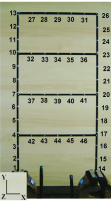
In this experiment, a steel structure constructed in the laborato-ry was used, following the parameters presented in table 1. The structure was fixed by mechanical clamps to simulate a crimping and ensure the boundary conditions in the supports during the measurements. The structure assembly is shown in figure 5. 46 points were measured for vertical and horizontal vibration modes. The transverse modes were not evaluated in this work.
Figure 2
Vibration of a beam induced by a fluid flow:
boundary conditions and geometry
Source: Dettmer e Peric, [13]
Figure 3
Finite volume mesh for the fluid domain
Figure 4
Finite element mesh for the structure domain
Table 1
Properties of steel structure
Properties of steel structure Numeric values
Height (H) 0.6 m
Partial height (D) 0.15 m
Section thickness (a) 0.00615 m
Section lenght (b) 0.0131 m
Density of mass (ρ) 7,850 kg/m3
Young module (E) 200 GPa
Poisson module (υ) 0,26 –
Cross-sectional area (A = a.b) 8.06 x 10 -05 m2
3.2.2 Experimental procedure
Data was acquired using a dynamic vibration analyzer, Figure 6b. The sampling frequency was fixed at 400 Hz. The input and output signals were filtered through a power window and an exponential decay window respectively, while the resolution of the measure-ment was 0.25 Hz.
The structure was excited with an impact hammer (Figure 6b) at node 24, pushing it into the negative direction of the x-axis. The hammer has a load cell with a sensitivity of 2.27 mV/N to detect the magnitude of the excitation force.
The vibration response was measured at all nodes with an acceler-ometer. The accelerometer was positioned in the structure to mea-sure only the accelerations perpendicular to the surface thereof (Figure 6a).
The RFP method was implemented and inserted into the EasyMod
toolbox (Kouroussis, [18]). Thus, it was possible to obtain the ex-perimental modal parameters.
3.3 Coupled fluid-structure problem
The case analyzed in this work has the objective of studying the dynamic behavior of a structure subjected to oscillations of pressure loads. To simulate this, a rigid cube-shaped body is submerged in an air flow, generating vortices which, conse-quently, make the lift coefficient on the structure oscillate. To compare with the vibration modes of the structure, a modal analysis was performed through the ANSYS® software, where the modes of vibration and natural frequencies for several simi-lar porticos with different sizes and rigidities were determined. Table 3 gives a summary of this study, while Figure 7 shows the structure and its main dimensions.
It is noticed that the natural frequency of the structure is changed as its dimensions change. For example, a portico 120 cm high by 60 cm wide, made with 0.615 x 1.31 cm cross-section bars, has a natural frequency close to 7.8 Hz. This was the portico used in the coupled fluid-structure problem simulated and figure 8 shows the model and the boundary conditions.
A similar approach to the case of fluid-structure coupling in section 3.1 of this work was considered. That is, a mobile mesh for the fluid in the region near the structure, constant air inflow, non-slip condition at the contacts between fluid and solid bodies and zero pressure at the outlet. For the generation of the vortices, the flow was blocked by a rigid square shaped body with 100 cm sides, as was the case of the beam being excited by the fluid flow (item 3.1 of this article). Considering that the lift coefficient generated by the rigid obstacle oscillates
Figure 5
Steel structure used for the experiment
Figure 6
(a) Position of the accelerometer and (b) Vibration
analyzer and impact hammer
(a)
(b)
Table 3
Natural frequencies for the first mode of vibration
of the various frames tested by the FEM
H x L (mm)
a x b (mm)
Natural frequency of 1st vibration
mode
1200 x 600 6.15 x 13.1 7.8
1200 x 600 12.3 x 26.2 15.9
1800 x 900 18.4 x 39.3 10.6
2400 x 1200 24.6 x 52.4 7.9
2700 x 1350 27.7 x 58.9 7.1
3000 x 1500 30.8 x 65.5 6.4
Table 2
Natural frequencies for the first three modes
of vibration
Method RFP FEM Frequency
[Hz]
Damping coefficient
[%]
Frequency [Hz]
1st 26,302 1,2746 29,319
2nd 92,508 0,2440 98,771
between positive and negative, the portico was positioned “ly-ing down” and set at its right end to cause the lift coefficient to act in a way to oscillate the structure according to its modes of vibration analyzed.
Here, the velocity of entry was controlled and some velocities were tested, monitoring the drag and lift coefficients for each of these velocities. For a velocity u∞ = 80 m/s it was found that the oscillation frequency of the lift coefficient on the portico is close to 8 Hz, as well as the natural frequency of the portico. For the fluid, a mesh of 21,162 elements and 21,450 nodes was assembled, whereas for the structure, a mesh of 1,082 elements and 10,192 nodes was constructed. In Figures 9 and 10, the meshes for the fluid domain and structure are respec-tively shown.
4. Results and discussions
This section will present the results of each of the models pre-sented in the previous section, as well as the relevant discussions.
4.1 Vibration of a beam induced by a fluid
The displacement along the vertical direction of the vertex on the right side the beam was monitored. The results obtained by Dett -mer and Peric [13] and Wall and Ramm [12] are shown in figures 11 and 12, respectively.
In both cases, the amplitude of the vertical displacement is close to 1.2 cm, while a cycle takes around 0.3 s. It is noticed that the behavior for the two cases are not identical, mainly at the begin-ning of the flow, which is in transient state. This because each au-thor has developed their own numerical model for the resolution. However, what is noticeable is that after establishing the steady state, the dynamic behavior of the structure is the same.
During the resolution of the coupled problem simulated by the au -thors of this article, the drag (Cd) and lift (Cl) coefficients on the structure were monitored in addition to the beam displacement. The drag and lift oscillations are shown in Figures 13 and 14. It is
Figure 7
Structural model with its main measurements
of the porch used for modal analysis study
Figure 8
Geometry for the coupled problem
Figure 9
Finite volume mesh for the coupled problem
Figure 10
noted that a variation cycle of the Cl takes approximately the same 0.3 s as the oscillation cycle of the beam.
The displacement obtained in the simulation of this problem is also in agreement with the works found in the literature, which is shown in Figures 15 and 16. The oscillation of the beam during the steady flow state of the fluid is shown in Figure 17.
4.2 Modal analysis of a small-scale steel structure
The natural frequencies and damping factor for the first three modes of vibration are shown in Table 2, where only the modes in the x-y plane were measured, the other planes being
disre-garded. Regarding the FEM, the results of the natural frequencies of the first, second and third modes of vibration using the RFP method present an error of 10.3%, 6.3% and 7.4%, respectively.
Figure 11
Vertical displacement of the vertex of the structure.
Results obtained by Dettmer and Peric [13]
Figure 12
Vertical displacement of the vertex and
the center of the structure. Results obtained by
Wall and Ramm [12]
Figure 13
Drag coeficient between 13 and 14 seconds
of simulation
Figure 14
Lift coeficient between 8 and 9 seconds
Figure 15
Displacement of the right vertex of the beam
over time
Figure 16
Figure 17
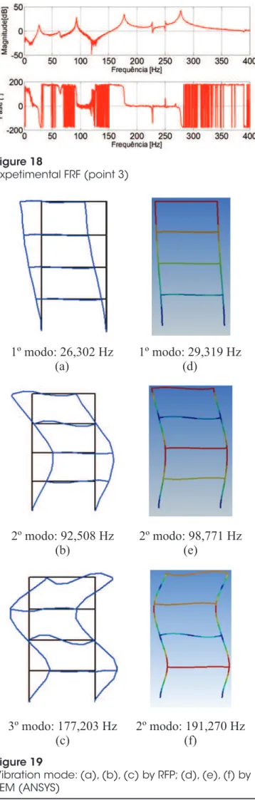
Figure 18 shows the experimental Frequency Response Function (FRF) of point 3.
Figure 19 shows the vibration modes obtained by the RFP method with the experimental data and by the FEM using the ANSYS® software.
As shown, the results obtained by the RFP method are compat-ible with the FEM, although the natural frequencies have a small dispersion in the values when the two methods are compared. This can be attributed to the following factors: geometric divergences between the actual portico and the modeling in the analytical meth-od; the result obtained by the FEM does not consider the damp-ing factor; the RFP method suffers external influences that are not controllable at the moment of data collection, interfering with the final results.
The validation of the numerical modeling used by the ANSYS® software was effective when comparing its results with the
experi-Figure 18
Expetimental FRF (point 3)
Figure 19
Vibration mode: (a), (b), (c) by RFP; (d), (e), (f) by
1º modo: 26,302 Hz
(a)
2º modo: 92,508 Hz
(b)
3º modo: 177,203 Hz
(c)
1º modo: 29,319 Hz
(d)
2º modo: 98,771 Hz
(e)
2º modo: 191,270 Hz
(f)
Figure 20
Lift coefficient on the Portico x Time
Figure 21
mental results. In this way, numerical modeling was used to per-form the modal analysis of the structure presented in the sequence of this work.
4.3 Coupled fluid-structure problem
In this study, it was sought to balance the frequency of oscillations of the lift coefficient with the natural frequency relative to the 1st mode of vibration of a portico. The portico chosen and the problem were those previously modeled.
The drag coefficient in this case is not important, since the verti-cal displacement of the upper left vertex of the portico was mon-itored. The interesting thing is the behavior of the lift coefficient on the portico, which is responsible for the vertical displace-ments on the structure. Figures 20 and 21 show the behavior of the lift coefficient, which varies with average null value and with amplitude of up to 0.075. Its oscillation frequency is close
to 8.8 Hz, according to its Fast Fourier Transform (FFT) shown in figure 22.
The graph of the FFT for the lift coefficient shows that the oscilla-tion frequency of this is 8.8 Hz. This frequency is very close to the natural frequency of the analyzed portico, which is 7.9 Hz. One can imagine that the portico is vibrating according to its first mode of vibration.
To verify this, it is necessary to analyze the behavior of the portico displacement. The vertical displacement of the upper left vertex is shown in Figures 23 and 24. Finally, in Figure 25, it can be seen that the frequency taken from the FFT of the actual displacement of the structure registers a frequency of 8.8 Hz, as well as that of the lift coefficient.
In this case, it was observed that the displacement increases in
Figure 22
FFT for the Lift coefficient
Figure 23
Displacement of the Upper left vertex x Time
Figure 24
Displacement of the Upper left vertex between
3 and 6 seconds
Figure 25
amplitude in each cycle until a certain moment, reaching a maximum displacement around 17 centimeters. After reaching this maximum amplitude, it begins to decay again, and this amplitude variation per-sists until the steady state is established. Figure 26 illustrates this behavior. Furthermore, in this figure, it is observed that the structure vibrates according to its first mode of vibration, and also that the am-plitude of the displacement increases in each cycle up to 4.32 onds, then gradually decreases up to 4.45 seconds. After 4.50 sec-onds, the amplitude starts increasing again and so on until the steady state is reached.
5. Conclusions
In this work, a coupled fluid-structure problem was approached, com-paring the result with the modal analysis of a structure. For this, an experimental and numerical approach was performed, that is, the ex-perimental results were used for validation of numerical modeling. The conclusions of each case addressed in the paper are presented below.
5.1 Vibration of a beam induced by a fluid
After performing a comparative analysis of a problem found in
the literature, it is concluded that the model adopted for solving a coupled fluid-structure problem, where the structure is flexible and the Newtonian fluid, presents results compatible with the numerical models developed in the references. This model is adopted by AN-SYS® multi-physical analysis software, used in case simulations.
5.2 Modal analysis of a small scale steel structure
As presented, the results obtained by the RFP method are compatible with the FEM, although the natural frequencies have a small dispersion in the values when the two methods are compared. This can be attrib-uted to the following factors: geometric divergences between the actual portico and the model in the analytical method; the result obtained by the FEM does not consider the damping factor; the RFP method under-goes external influences that are not controllable at the moment of data collection, interfering with the final results. These results validate the nu-merical modeling used in the ANSYS® software. Therefore, it is valid to use this for modal analysis of the structure approached in the next case.
5.3 Coupled fluid-structure problem
The coupled problem consists in analyzing the dynamic behavior
Figure 26
of the structure when it is subjected to an oscillatory lift coefficient, generated by the incidence of an airflow in obstacles. It was veri-fied that a structure submitted to this type of flow tends to move according to its modes of vibration.
Finally, it is added that the advancement of computational mechan -ics is allowing the resolution of complex problems in a timely man-ner and this can be incorporated into structural projects. There is still a long and arduous path of research to be done to make this habitual. However, it is believed that the consideration of the dy-namic effects in light structures can bring more accurate results of the phenomena that involve these structures, and make them safer and more economical at the same time.
6. Acknowledgments
The authors of this paper thank UTFPR – Federal University of Technology – Paraná – Pato Branco Campus – Pato Branco Cam-pus, for the resources available to carry out this research and CAPES, for financial support to the first author. The authors would also like to thank the Araucária Foundation for Support for Sci-entific and Technological Development, for the financial support granted – Notice 24/2012 Basic and Applied Research Program (FUNTEF-PR 376/2014).
7. References
[1] Souza JR., L. C. Uma Aplicação dos Métodos dos Elemen-tos FiniElemen-tos e Diferenças Finitas à Interação Fluido-Estrutura. Dissertação de Mestrado em Estruturas e Construção Civil, Publicação E.DM-008/06, Departamento de Engenharia Civil e Ambiental, Universidade de Brasília, DF, 2006, 197p. [2] Gilbert, R. J. “Vibrations des structures – Interactions avec
les fluids – Sources d´excitation aléatoires”. E. Eyroller, Par-is, França, 1988.
[3] Zienkievicz, O. C. e Taylor, R. L. “The Finite Element Method”, Fourth Edition, McGraw-Hill, Pub. Co. Ltd. UK, vol.2, 1989.
[4] Junger, M.C. “Acoustic fluid-elastic structure interactions: basic concepts.” In: Computers & Structures, vol. 65, nº 3, 287-293, 1997.
[5] Tabarrok, B. “Dual formulations for acoustic-structural vibra-tions.” In: International Journal for Numerical Methods in
En-gineering, vol. 13, 197-201p, 1978.
[6] Leitão, G. B. Análise Numérica de Segunda Ordem de Pór-ticos Planos de Estruturas de Aço. Dissertação de Mestrado em Estruturas, Curso de Pós Graduação em Engenharia Civil, UNICAMP, Campinas, SP, 2014.
[7] Everstine, C.G. “Finite elemento formulations of structural acoustics problems.” In: Computers & Structures, vol. 65, nº 3, 307-321p, 1997.
[8] Gomes, F.A.A. Análise Numérica do Escoamento Hipersôni-co em Torno de Corpos Rombudos Utilizando Métodos de Alta Ordem. Tese de Doutorado – Instituto Tecnológico de Aeronáutica, São José dos Campos. 2012.
[9] Soares Jr, D. Análise Dinâmica de Sistemas Não-lineares com Acoplamento do Tipo Solo-fluido-estrutura por Intermé-dio dos Métodos dos Elementos Finitos e do Método dos
Elementos de Contorno. Tese de Doutorado em Engenharia Civil – Universidade Federal do Rio de Janeiro, 2004. [10] Bazilevs, Y., Takizawa, K., and Tezduyar, T. E.
“Computa-tional fluid-structure interaction: methods and applications”.
John Wiley & Sons. 2013.
[11] Zienkievicz, O. C. e Bettess, P. “Fluid-structures dynamics interaction and wave forces. An introduction to numerical treatment. International Journal for Numerical Methods in
Engineering, 13.1, 1-16p. 1978.
[12] Wall, W. A. e Ramm, E. “Fluid-structure interaction based upon a stabilized (ALE) finite elemento method”. Compu-tational mechanics. New Trends and Applications. S.R. Idelsohn, E. Oñate and E.N. Dvorkin (Eds). CIMNE, Barce-lona, Spain, 1998.
[13] Dettmer, W., Peric, D. “A computational framework for fluid-structure interaction: Finite elemento formulation and appli-cations”. Computational Methods Appl. Mech. Engrg. 195 5754-5779, 2005.
[14] Teixeira, P. R. F. e Awruch, A. M. “Numerical simulation of fluid-structure interaction using the finite elemento method”. Computers & Fluids. 34, 249-273, 2004.
[15] Ewins, D. J., 2000. “Modal Testing: Theory, Practice and Ap-plication”. John Wiley, Philadelphia, 2nd edition.
[16] Schwarz, B. e Richardson, M. H. “Experimental Modal Anal-ysis. In: CSI Reliability Week, 1999. Proceedings: James -town, Califórnia, 1999.
[17] FLUENT v6.3, Fluent Incorporate Inc., Centerra Resource Park, 10, Cavendish Court, Lebanon, New Hampshire, USA, 03766, 2006.