OpRisk: The challenges of Basel Advanced Approach
Carla Sofia Santos Carloto
A Dissertation presented in partial fulfillment of the requirements for the Degree of Master in Finance
Supervisor
Prof. Miguel Ferreira, Prof. Associado, ISCTE Business School, Finance Department
Abstract
Operational Risk is defined by Basel Committee as “the risk of loss resulting from inadequate or failed internal processes, people and systems or from external events.” Since the beginning, all institutions know that operational risk is present in their activities, but just when Basel Committee introduced as mandatory to have regulatory capital requirements, institutions change their focus from Credit Risk and Market Risk to manage operational risk as a way to reduce regulatory capital.
To present some alternative models to be support Advanced Approach, I investigate possible approaches and available statistical distributions that better explain factors/variables like operational risk losses using public data.
From the reports published by ORX and FED, I simulate capital requirements using different distributions for each Business Line and Event type, and compare final results and behaviors.
The important conclusion of this paper is that is critical to consider all four elements to build a soundness model to estimate capital needs with internal models. The model should be suitable for the reality of institutions rather than be evaluated as the best in statistical measures. More than be regulatory requirement these internal models should be considered an important tool for risk management.
JEL Classification: G32
Keywords: Operational Risk, Monte Carlo Simulation, Basel II, Capital Adequacy Model for Operational Risk
Data availability: The data used in this dissertation are public and can be consultant in Organizations/Institutions Sites.
Resumo
Risco Operacional é definido pelo Comité de Basileia como o “Risco de perdas em resultado da inadequação ou falha de processos internos, pessoas, sistemas ou eventos externos”.
Desde sempre que as Instituições tem conhecimento da existência de Risco Operacional, mas apenas quando o Comité introduziu como requisito obrigatório no cálculo de capital regulamentar, que as instituições alteraram o enfoque da sua gestão de risco do Risco de Crédito e de Mercado para a gestão do Risco Operacional para optimizarem o capital regulamentar.
Para apresentar modelos alternativos de suporte à Abordagem Avançada do ponto de vista quantitativo, investiguei possíveis abordagens e distribuições estatísticas que melhor explicassem os acontecimentos de risco operacional recorrendo a dados públicos. Dos relatórios publicados pela ORX e FED, simulei os requisitos de capitais por cada Linha de Negócio e Tipo de Evento recorrendo a diferentes distribuições e comparando os resultados finais, assim como, o comportamento das mesmas.
A conclusão importante deste estudo é que é crucial considerar os quatro elementos para a construção de um modelo interno robusto para estimar as necessidades de capital. O modelo deve reflectir a realidade das instituições e não apenas obter melhores medidas estatísticas em relação à sua qualidade. Mais do que um requisito regulamentar, os modelos internos devem ser considerados uma importante ferramenta para a gestão de risco nas instituições.
Classificação do JEL: G32
Palavras-chave: Risco Operacional, Simulação de Monte Carlo, Acordo de Basileia II, Modelo de Adequacidade de Capital de Risco Operacional
Disponibilidade de dados: Os dados utilizados na dissertação são públicos e podem ser consultados nos sites das Organizações/Instituições
Acknowledgements
I dedicate this study to my family and friends for their support and encouragement. I would like to thank to my supervisory on this study, Professor Miguel Ferreira for his superior orientation on the work presented
INDEX
1. Introduction ... 1
2. Theoretical framework ... 5
2.1 Basel II and Committee’s recommendations for Operational Risk... 5
2.1.1 BASIC INDICATOR (BIA)...6
2.1.2 STANDARDIZED APPROACH...6
2.1.3 ADVANCED MEASUREMENT APPROACHES (AMA)...9
2.2 Measurement Models for Operational Risk... 12
2.2.1 INTERNAL DATA...12
2.2.2 EXTERNAL DATA...22
2.2.3 SCENARIO ANALYSIS...23
2.2.4 BUSINESS ENVIROMENT...24
2.2.5 INTEGRATION TECHNIQUES...26
3. Application Monte Carlo Simulations and Capital at Risk ... 30
4. Data Description ... 35 4.1. FEDERAL 2004... 35 4.2. ORX Report 2007... 36 5. Conclusions... 38 6. References... 44 7. Bibliography... 45 Appendix... 48
1 1. Introduction
In a time when once again the financial system is going through a crisis, is also the time of Basel II rules are beginning to be mandatory in several financial systems. Operational risk is the newest requirement introduced by the Committee with Basel II Accord and has become a fundamental part of every institution risks management strategy. Basel document by itself has no mandatory enforcement, so it was necessary for European Union to transpose and make minor changes and publish CRD (Capital Requirements Directive) in October 2005.
2008 is year zero for institutions to start to use this new framework, and Operational Risk appears to be the major challenge due to lack of historical sound data and experience in building models the same way that institutions have been doing in the past years to Credit and Market Risk. These models were used only for internal management proposals and now institutions can use them to calculate regulatory capital.
The Committee define major principals for operational risk management framework and advice supervisors how to validate internal models, but has not yet been sensitivity to define values and detail approaches.
The new framework presents several available approaches which allow institutions to adopt the one that best fits their risk profile and risk management strategy. The main objective of three available approaches is to provide incentives for institutions to improve their risk-management practices, with more risk-sensitive risk weightings as institutions adopt more sophisticated approaches to operational risk management.
For institutions the first challenge is to decide their own definition of operational risk and their scope with the question of including legal and reputational risk. They have to plan their strategy for risk management by choosing which approach to adopt and the next steps to implement a more complex framework, allow reducing regulatory capital allocated to operational risk as management process becomes more effective and sound.
2 The available approaches for operational risk are Basic Indicator (BIA), Standard Approach (STA) and Advanced Measurement Approach (AMA), and in each one are defined quantitative and qualitative requirements that institutions must be compliant with.
With respect to the AMA Approach, the major challenge is sound information with minimum historical of three years. To build a sound internal model is necessary information to allow shaping the better statistical distribution that explains the events and will permit to estimate losses with 99,90% of confidence level. Institutions must implement the loss data collection process and guarantee completeness and timeliness of this process.
This paper explores theoretical models available from other risk management models like Actuarial model for insurance risk provisions. I apply one approach to aggregate loss data collected from public reports. I simulate and build Aggregated Loss Distribution for each business line and event type and estimate Capital at Risk according to distributions results.
After introducing the regulatory principles, this paper presents measurement models for operational risk quantification. An operational risk model should include Internal Data, External Data, Scenario Analysis and Business Environment. Institutions must define their framework for each part of the model and how to integrate the different techniques used.
For the loss data collect, institutions should use a technique that best fits the available loss data. The most common techniques are: Empirical Loss distributions, Parametric Loss Distributions, Actuarial Models and Extreme Value Theory.
Empirical Loss Distributions and Parametric Loss Distributions are Total Loss Techniques meaning that they do not separate severity from frequency. In contrast, Actuarial model is a technique of Aggregated Loss and considers severity and frequency as two separated input factors.
3 Historically the major operational risk events are characterized by higher severity and low frequency and for statistical modeling of these events, the Extreme Value Theory is very useful. This technique allows modeling the right tail of an Aggregated Loss Distribution without compromise the distribution’s principal modeling process.
After choosing the internal data treatment methodology, the institutions must use external data to adjust their estimates. External data can be used only as quality data or be integrated in the modeling process. When used is necessary to make adjustments through data treatment and define which technique to use to integrate both data in the same model.
Adopting the Advanced Approach implies the use of business factors on model calibration. This calibration can be made indirectly through scenario analysis or directly recurring to direct calibration with Q factor build using score functions.
As mentioned before, data integration is very critical and I identify several methodologies to be applied to the process of data integration and Bayesian Integration or Integration by convolution are the ones that best fits the needs of data modeling for Operational Risk.
Other possibility is to integrate output data instead of input data applying either weighting average Capital at Risk estimated in each intermediate steps (e.g. LDA, External data) or considering the first output and then add next results using adjustments factors.
The final step is this framework is to build a matrix of estimated Capital at Risk for each business line and event type, and once again there are available several techniques assuming that losses are independent.
In this paper I apply Loss Data Aggregation methodology to published data from FED and ORX, and it is possible to generate as output Capital at Risk for each business line and event type, and compare results between studies, statistical distributions and input data presented with detail. The methodology and results are presented in sections 3 and 4 of the paper, detailed data, indicators and graphs are presented in the appendix.
4 It is not possible to compare the three approaches (BIA, STA and AMA) between themselves because it is not available about participants and their historical individual losses, so this paper focuses in how to build the quantitative framework for Advanced Measurement Approach for Operational Risk.
At the same time as this study was prepared, Basel Committee published the 2008 LDCE for Operational Risk, where is presented the set of methodologies implemented by institutions. When comparing both documents is understandable that the methodologies proposed and implemented are similar and also some institutions use the same statistical distributions building models that better fit their reality and their historical data.
The diversity of results obtained demonstrate that soundness information and their completeness is the challenge for all institutions, for building a strong internal model of Operational Risk that aims not just risk management but also helps institutions to mitigate risks and incentive them to implement advanced approaches as a path to adjust regulatory capital to their own risk profile.
The main conclusion from the results is that is necessary to consider all four elements [Data (Internal and external), scenario analysis and business environment] to build a soundness internal and the critical factor of success is the quality of data collected during the previous years.
5 2. Theoretical framework
2.1 Basel II and Committee’s recommendations for Operational Risk
Operational risk is introduced by Basel II as mandatory requirement for capital adequacy of financial institutions and this framework has been adopted by almost all supervisors. Basel II is a challenge for banks and their supervisors, because of the advanced approach to calculate minimum capital requirements.Operational risk is defined in the document “as the risk of loss resulting from inadequate or failed internal processes, people and systems or from external events. This definition includes legal risk, but excludes strategic and reputational risk.” Notice that “legal risk includes, but is not limited to, exposure to fines, penalties, or punitive damages resulting from supervisory actions, as well as private settlements.”
To help institutions and their supervisors, BIS also publish a document with recommendations about operational risk management: “Sound Practices for the Management and Supervision of Operational Risk”. In this document there are ten best practices to orient institutions to create their own framework and to help supervisors to evaluate presented methodologies.
The document presents a framework with three possible approaches to calculate capital charge and to manage operational risk according with calculation methodology chosen. Operational risk framework defines the following approaches:
1) Basic Indicator Approach;
2) Standardized Approach ( also available “Alternative Standardized Approach”); 3) Advanced Measurement Approaches (AMA).
There are two major differences between approaches related with calculations method and mandatory quality requirements associated to those methods. As the complexity of calculations increases the management requirements also increase because internal data becomes fundamental to the framework.
6 2.1.1 BASIC INDICATOR (BIA)
In the first approach the capital charge is 15% of annual gross income (average of last three years with positive income) and recommends institutions to comply with “Sound Practices for the Management and Supervision of Operational Risk”.
The capital requirements are given by:
where:
= capital charge under the Basic Indicator Approach for Operational Risk; GI = annual gross income of the last three years (if all positive);
N= 3 if all previous years the gross income is positive; α = 15% which is set by the Committee.
As Gross Income could have several interpretations, the Committee defines GI as the sum of net interest income and net non-interest income. This measure should be gross of any provisions and gross of operating expenses including those related to outsourcing service providers. Any profit or loss related to: sale of securities in the banking book, extraordinary items and related to insurance should be excluded from this measure.
2.1.2 STANDARDIZED APPROACH
The second approach allows institutions to calculate capital charge according with their business lines, because the Committee defines different charge for each business line. The gross income is used as an indicator to determine the scale of business activity and therefore an estimative of operational risk exposure.
The first step is to segment institutions gross income into eight business lines: 1) Corporate Finance;
7 3) Retail Banking;
4) Commercial Banking; 5) Payments and Settlements; 6) Agency Services;
7) Asset Management; 8) Retail Brokerage.
The capital charge is calculated as follows:
where:
= capital charge under the Standardized Approach for Operational Risk;
= annual gross income of the last three years (as defined above) for each business line;
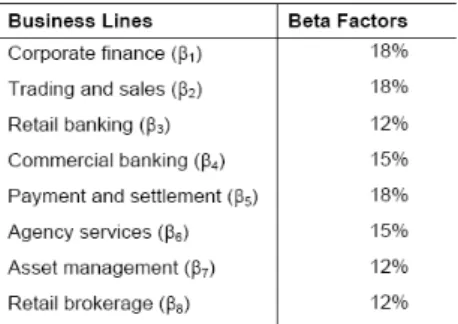
= a fixed percentage, set by the Committee, relating the level of required capital for each business line. The values of Betas are:
Figure 1: Beta coefficients (Standardized Approach)
The proposal values for Beta’s is meant to be used as an estimated factor supported in industry-wide operational risk loss experience and the aggregated level of gross income in each business line.
Note that the Committee intends to review the calibration of Betas (and Alpha for Basic Indicator) when more risk data are available to support the calibration process.
8 The Committee also refers that national supervisors can authorize institutions to adopt Alternative Standardized Approach. The calculations are equal to what is present expected to Retail Banking and Commercial Banking. For these two business lines the formula can be:
where:
= capital charge under the Standardized Approach for Retail Banking; = Beta for Retail Banking business line;
= last three years average of total outstanding retail loans and advances with any adjustment provided by risk weight or by provisions. In the full document is defined what can be considered to build this indicator.
= 0,035 (value defined by the Committee)
For a risk management point of view, the Committee is more demanding in this approach and Sound Practices became mandatory to be implemented and supervisors must be more meticulous on acceptance process of institutions choices.
The Committee is clear when defining as mandatory an implementation of a governance model for operational risk management that must include the following topics:
• Top management involvement;
• Organizational structure and Operational Risk Management Processes ; • Operational Risk Management Policy;
• Definitions and glossary for Operational Risk;
• Criteria for Mapping the Gross Income into eight business lines; • Incentive systems to sound risk management.
This governance model should guarantee that Operational Risk Management function includes the definition of identification, assessment, monitoring, control and mitigation of operational risks.
9 Because more advanced methodologies depend on information collected by institutions and their historical data, this approach introduces the process of risk identification and measurement usual known as Loss Data Collection and uses important tools like Scenario Analysis and periodic Risk Self Assessments.
For the Committee and local supervisors is fundamental reporting about real operational risk losses, which in a first level should occur internally to Top Management and business units (if applicable) and then externally to supervisor.
The reporting process should comply with the following principles: • Completeness: comprehensive set of collected losses.
• Timeliness: time proximity of the recorded information to the loss event. • Accessibility: cost of getting the information.
• Quality and quantity of information collected Date, nature and amount of loss, etc. Exposure information.
Rating information.
The Risk Assessment process must guarantee that all relevant operational risk data like material losses occurred are included in assessments and this tool is important to the management process and for the definition of the institution risk profile.
All processes referred before must be documented and be well known by all institution’s employees and be reviewed and validated by independent department (internal audit). Even with an internal review process implemented the operational risk management process must be subject to regular review by external auditors and/or supervisors.
2.1.3 ADVANCED MEASUREMENT APPROACHES (AMA)
Under this approach the regulatory capital requirement is calculated by their internal operational risk management system, which needs approval by national supervisor. The requirements in this approach include all mentioned for the Standard Approach, and add some additional qualitative and quantitative criteria.
10 The most important is that when an institution adopts a more advanced approach it can not go back if the regulatory capital requirements are bigger than if using Standard approach.
For adopting this approach is necessary for a period of time to be under supervisor monitoring, which will allow the supervisor to determine if the internal approach is appropriated and credible. The most important is that the internal measurement system estimates reasonably well operational risk unexpected losses based on the combined use of data about internal losses calibrated with relevant external losses, and use of scenario analysis adjusted with information from business environment and internal control factors.
The system should be capable of allocating economic capital for operational risk in each business line to be an incentive to improve individual operational risk management of business lines.
In terms of quantitative standards the Committee has not specified the approach or any distributional assumption for the measurement system. But the institution must demonstrate to the local supervisor that the internal model captures severe “tail” loss events and be comparable to one year holding period and a 99.9th percentile confidence interval like it is happens in internal ratings based approach for credit risk.
In the development of an internal measurement system, institutions must have and maintain rigorous procedures that will allow an independent validation. The Committee will review industry practices and the levels of capital requirements estimated by AMA and redefine its proposals if appropriate.
The document presents a series of quantitative standards:
• The internal risk measurement must be consistent with Operational risk definition and the loss events types defined in the document;
• An institution should calculate its regulatory capital requirements as the sum of expected loss and unexpected loss;
11 • The internal system must be sufficiently granular to capture the drivers that
affect the shape of the tail of the loss estimates.
• Risk measures for different operational risk must be added for determining the regulatory capital, but institutions can use correlations determined internally, if the methodology used is sound, implemented with integrity and approved by national supervisor.
• Must have certain features like the use of internal data, relevant external data, scenario analysis, business environment and internal control systems.
• All system must be well documented, must be credible and transparent. All features mentioned before should be weighted in the system and this must be verifiable by independent entities and supervisor.
The Basel document in following sections presents the principles for each key feature to orient institutions and supervisors for what is expected to be an internal system to measure operational risk.
For capital requirement it is allowed to use risk mitigation like insurances. The Committee has limited to 20% of total capital charge calculated the use of insurances and institutions must be complying with several criteria presented.
In practice it allows institutions to adopt partially Advanced Approach to some parts of its operations and a less advanced approach for the balance sheet if the conditions defined in the document are met.
12
2.2 Measurement Models for Operational Risk
The document published by the Committee only presents general principles for building a sound system for measuring operational risk and in the following sections are available methodologies to accomplish the several features necessary to have an internal system. 2.2.1 INTERNAL DATA
When an institution decides to adopt the AMA approach for the treatment of operational risk, it is need to be compliant by developing their own model based on internal and external data, developing scenarios analysis and integrating information from business environment and internal control.
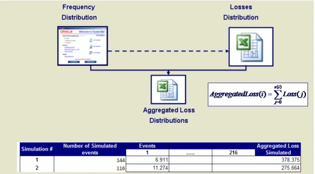
If institutions collect 3 to 5 years of historical data about operational risk events, they will be able to use a methodology denominated “Loss Distribution Approach”. This approach assumes that using the data it is possible to build 2 distributions:
1. Frequency distribution, and 2. Severity distribution.
The next step is to aggregate both distributions using Monte Carlo simulation resulting in one distribution, the Aggregated Loss Distribution (ALD).
This distribution permits to use several statistical techniques to estimate operational risk losses, and estimate the level of capital needed to be compliant for operational risk. The most common techniques used in this methodology are:
1. Empirical Loss distributions; 2. Parametric Loss Distributions; 3. Actuarial Models; and
4. Extreme Value Theory.
Typically using this approach the results are more reliable from a mathematical point of view. But this affirmation can be questioned, being only valid when the data used permits. It is necessary that we are aware that the event collection is new and that
13 majority of the institutions are having problems in collecting data needed for the modeling process. This is a newly process and the historical data collect can be insufficient or their quality can be questionable.
EMPIRICAL LOSS DISTRIBUTIONS
The quantitative analysis of Operational Risk can be done using empirical loss distributions, known as empirical simulation technique. An important reminder is that this technique do distinguishes between frequency and severity loss distribution for loss events (Total Loss Approach).
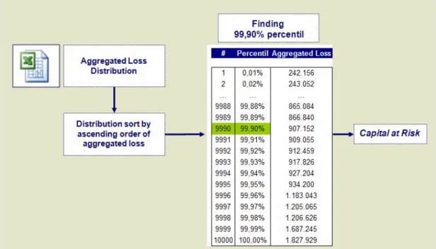
This technique consists in collecting internal data of losses occurred during a period of time, sorted by ascending order of loss amounts and estimating VaR for a particular confidence level; using the Basel Regulation the confidence level is 99, 90%.
According to the Basel Rules, this technique requires:
1) The collection of 5 years of data of losses related with operational risk events; 2) Analyze the data to determine loss distribution, meaning calculating the
frequency of each loss level. For improving data quality it is possible if relevant to remove inflation effect or some seasonal effects present in data.
3) The final step is to identify the loss distribution’s quantile and corresponding loss value. This quantile is defined by the confidence level, and the amount is the estimative for “Capital at Risk” calculated only with historical data.
14 In short the most important advantages and disadvantages of this technique are:
Advantages Disadvantages
Intuitive Method All estimations are made assuming that
historical losses are a good indicator for predicting future losses, meaning that the risk management process keeps equals, and this is difficult to guarantee.
Permits calculations without considering the statistical distribution of the underlying phenomenon, the loss events. This simplifies calculation and reduces time to produce results.
This technique assumes that future losses will have the same behavior of past losses.
It is necessary a large set of data with a certain number of losses.
PARAMETRIC LOSS DISTRIBUTIONS
In contrast to the empirical loss distribution, this methodology does not uses historical data to estimate operational risk losses. Historical data only provides the theoretical distribution parameters that best fit the underlying phenomenon.
This methodology also is a technique of Total Loss.
If for Market Risk is common to assume returns normality, for Operational Risk that assumption is not valid because of the low frequency of events, the large number of events with a low loss amount, and the reduced number of events with a high loss amount. Given these facts the distribution chosen should be an asymmetric because it fits better this kind of data.
15 1) Data collection and treatment for removing external effects mentioned above. It should be created a set of theoretical distributions, from which is chosen the distribution that best support the modeling process. All distributions considered in this stage are asymmetric and with slight right tail (e.g. Log-Normal, Weibull, Gamma)
2) Next step is to identify a distribution that best fits losses behavior. One of the most popular methods is the quant-quantile graph that using data analysis compares sample’s quantiles with distribution’s quantiles.
3) For selecting a distribution, non-parametric tests can be used only for the sub-set selected in previous step.
The test is:
This test is expressed in terms of distance between the data distribution function and theoretical distribution.
4) And after selecting a distribution is necessary to estimate their parameters using the data collected in step 1. These parameters can be estimated using maximum likelihood method or moment’s method. With a full specification of distribution is possible to determine Capital at Risk (level of confidence of 99, 9%)
In summary the most important advantages and disadvantages of this technique are:
Advantages Disadvantages
Quantiles can be estimated using a minor data sample.
Can be difficult to select only one theoretical distribution for data adjustments.
Maximum Likelihood Estimators have important properties like has lower mean squared error.
Trying to obtain an adjustment for total data can cause bad estimations of right tail quantile (suggestion: Extreme Value Theory).
The data distribution is determinate statically and not only supported by exploratory data analysis.
In practice maximum likelihood estimators are difficult to calculate.
16 ACTUARIAL MODELS
For Operational Risk estimation is possible to apply actuarial models developed in the Insurance Industry. These kinds of models are built using two key factors/elements:
1) Number of Events – Frequency; 2) Losses Amount – Severity.
This methodology can be described in the following steps/stages:
1) Data collection and treatment, like in previous techniques but now is necessary to replicate data in 2 basis:
a. Frequency Table: Frequency along a time period;
b. Severity Table: Presented by ascending order of amounts.
2) Next step is selecting an adequate distribution for each phenomenon modeling. The statistical methods used are equal/ similar to what have been presented early. For Frequency is common use Poisson Distribution and for Severity is more typical choose Distribution like LogNormal, Pareto, Weibull or Gamma.
3) Build an Aggregated Loss Distribution considered aggregated loss a stochastic
process therefore , .
The aggregated loss distribution function can be calculated through a convolution operator using both distribution functions to produce a joint distribution function. In practice this operator is too complicated to implement and in alternative, institutions adopt an easier methodology based on Monte Carlo Simulations, ie:
(1) For example, considering that:
• Frequency = K a random variable Poisson Distribution • Severity = W a random variable LogNormal Distribution The following procedures are executed:
17 2) Random extraction of x random numbers from LogNormal
3) Repeating this process R times (R equal a number of Monte Carlo Simulations made).
The final result consists in a data sample with R dimension from where is possible to extract the adequate quantile value and determine CaR.
4) The last step consists in estimate ALD parameters, in case there is some evidence that the data are suppressed or truncated. It is possible that loss data does not exist or are uncompleted if the loss amount is lower than a certain value. For these situations, maximum likelihood estimators calculated without any adjustment can overestimate Capital at Risk.
One available alternative to solve this problem is the EM Algorithm (Dempser et al – 19771 and McLachlan and Krishnan - 19962). EM Algorithm consists in an interactive method that calculates maximum likelihood estimators using uncompleted data.
This method creates a hypothetic likelihood function, build on base of replacement of omitted values by values that are expected to follow the initial chosen distribution. In summary the most important advantages and disadvantages of this technique are:
Advantages Disadvantages
Based on math theories already proved that allow separated analysis of Frequency and Severity
Can be complicated to determine only one theoretical distribution for modeling the collected data
For identify Frequency and Severity Distributions are used Maximum Likelihood estimators
Assuming that loss amounts are identical distributed and independent from the number of loss events can be limiting,
18
Advantages Disadvantages
and is possible to produce less reliable results
Quantiles’ calculation is straight forward after estimating ALD parameters.
Trying to obtain adjustments for all data can cause a bad estimation for extreme values
The methods that use simulations can lead to not reliable results, mainly about quantiles calculations for aggregated loss distribution (this problem can be minimized by executing more simulations)
19 EXTREME VALUES THEORY
It is common to find extreme events when measuring any type of financial risk. This methodology has the objective to create models that capture situations whit low frequency but with high impact. This theory (EVT) allows us modeling the right tail of ALD without compromise the modeling of the distribution’s principal. By modeling a full distribution we incur in the risk of not modeling correctly not only the frequently events with lower impact but also the rare events with higher impact.
For Operational Risk Framework this method is extremely helpful as extreme losses are rare but with very large impact (the ones that have higher impact in business).
This method is implemented in three steps:
1) Data Collection: there are 3 major factors in this stage:
a. Time frame: It should be as long as possible for guarantee a major set of data;
b. Granularity level: It will depend on time frame scale and initial loss detail available;
c. Quality Data Analysis: Using available tools to evaluate their quality recurring to exploratory data analysis methods.
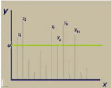
2) Next step consist in selecting a data sample with extreme values from the initial loss data set. For this it is available 2 methods: Block Maxima and Peaks-over-Threshold (POT).
Consider as a set of random variables with the following distribution functions . Each variable represents an operational loss in a specific time period.
The extreme values of the distribution right tail are those who verify the following condition: . This definition is according Block Maxima method, in which observations are divided by several categories being selected the maximum value as the extreme values of each one. With the selected observations we build a table to study according with asymptotic theory.
20 The alternative methodology “Peaks-over-Threshold” consist on previous definition of cut point for loss amount, and all values higher are considered extreme values (excess). Graphically, the selected processes of samples with extreme values are:
Figure 2: Block Maxima method Figure 3: Peaks-over-Threshold
3) The following step consists in defining the cutoff point using the POT method. It is necessary to consider a tradeoff between variance and distortion of parameters estimative. A correct method to do this tradeoff evaluation can be graphical analysis of the excess variability for each level of cutoff point.
Figure 4: POT – Example of graphical analysis of the excess
4) The final step is estimating parameters for the select distribution for those extreme values and identifies the specific quantile. Once the sample is set the asymptotic distribution of those observations can be one of the following, depending on the method used to build the sample:
21 (2) b. Generalized Pareto Distribution, GPD (Peaks-over-Threshold Method):
(3)
In summary the most important advantages and disadvantages of this technique are:
Advantages Disadvantages
Focus only on estimation of extreme values that are located on tails.
Asymptotic distributions are very sensitive to changes on parameters values.
Asymptotic distributions are available for these extreme cases.
22 2.2.2 EXTERNAL DATA
The use of external data is a requirement of the AMA approach in Basel II. This data can be used in two different methods:
• Scenario analysis as quality data (very conservative approach); • LDA approach as quantitative data.
For now, we are going to present only the second method because the first one will be detailed on a specific section.
Before including external data on the modeling process is necessary to define some elements:
1) Data treatment:
a. Linear adjustment: a unique coefficient is applied for adjusting data to institution dimension;
b. No-Linear adjustment: define specific coefficients for each type of event using regressions;
c. Data Filter: guarantee that only is used data form institutions with similar dimensions;
d. Not doing any data adjustment and integrate them on the modeling process. 2) How to join internal and external data:
a. Common usage: Aggregate external data to internal data base , creating a more robust base and apply previous presented methods;
b. Separated usage: Internal and external data are analyzed separately; creating a specific ALD just for this set of data, and after integrates both using one of following techniques: qualitative aggregation, aggregation throw linear combinatory, Bayesian aggregation or Convolution.
3) If the previous choice is common usage, then define how to treat losses amount: a. Aggregation made without consider loss amounts;
b. Aggregation made using loss amount criteria: internal data are used to model losses below a specific level and extremes for modeling loss above this level.
23 2.2.3 SCENARIO ANALYSIS
Nowadays one of the major problems that institutions face when try to model Operational Risk is the lack of information, either internal or external. This factor is critical for statistical estimation of event’s severity distribution.
According to Basel, institutions are obligated to use scenario analysis to validate or incorporate additional data to their previous results, mainly for extreme events. This is an alternative approach to Extreme Value Theory presented before.
The goal of the scenario analysis is to create fictional events, with the same event’s characteristics happened in the past, but due to lack of information are not included in the statistical analysis.
Scenario analysis is an important element for AMA approach in Operational Risk. These scenarios are building using empirical knowledge from institutions experts. This is a new reality for all institutions and is still in development in practical and in theoretical terms, and therefore somehow questionable.
This methodology can be summarized in figure below:
24 2.2.4 BUSINESS ENVIROMENT
For AMA implementation, a necessary requirement is adjusting results of modeling internal data using institution’s risk factors identified as cause of the loss events.
This information can be used in several levels:
• Indirect calibration when implement scenario analysis (methodology presented in above);
• Direct calibration (Q Factor) after aggregating LDA approach with scenario analysis.
For direct calibration, the necessary steps are:
1. Business environment and internal control mechanisms are defined by Top Management with a list of Key Risk Indicators (KRI’s);
2. Each KRI is classified considering his impact on Operational Risk using Scorecard;
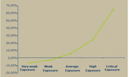
3. Capital at Risk is obtained in previous stages and adjusted using this new quality information.
This Scorecard is used to evaluate institution’s exposure to each KRI. For each exposure level is associated a relative weight. After consolidate all results is built a graph like this:
25 For a more conservative approach, weights can be adjusted using an exponential function, which means that factors with critical exposure will have an impact exponentially higher than factors where institutions have a lower exposure.
This coefficient is Q Factor and is used to adjust the CaR obtained before. This methodology includes the following steps:
• Collect information about the highest number of available KRI’s using self-assessments replied by High Management. This information is treated using univariate statistical techniques to determine discriminator capability of variables and to avoid inclusion of KRI correlated (Kruskal- Wallis Test, Discriminator Tree, and correlation analysis, among others).
• In case of collecting a large number of KRI’s should be considered the usage of techniques for sample dimension reduction to guarantee only the more relevant KRI’s in analysis (Principal components analysis or Factorial Analysis).
• Considered N business lines, and build a Score function for each one using a multiple linear regression:
(4)
Coefficients resulting from regression are each KRI associated weight. The Q-Factor is obtained with the sum up of all Scores in each Business Line:
(5)
The previous sum is obtained doing weighted sum considering relative weight of each business line on sample used for analysis.
26 2.2.5 INTEGRATION TECHNIQUES
• Input Aggregation
It is not possible to apply Aggregated Loss Distribution at all moments of data integration, especially in the input of data analysis.
As shown before, integration of internal and external data can be done by aggregating their distributions using the following techniques:
• Qualitative Aggregation – used generally when external data are also qualitative and heterogeneous (when their presentation is different from internal data format). This technique is based on estimating a parameter using qualitative data that will be used for adjusting quantitative data. The greater advantage is the technique’s simplicity, but in the other side is adjusting statistical outputs with parameters estimated based on qualitative data.
• Integration using Linear Combination is applied when both information sources are homogeneous. This technique consist on estimating factors which the sum is equal to one and weight both sources:
(6)
The main advantage is its linearity and the disadvantage is trying to combine qualitative factors.
• Bayesian Integration is the more valid method from the mathematician point of view, but more difficult to implement. Theoretically is based on Bayes Theorem :
(7)
This formula resumes using a priori information on the modeling process. When applied to Operational Risk, external data are a priori information available and using this method these data will adjust internal data results for creating a loss distribution a posteriori:
27 Figure 7: Methodology of Input Aggregation
This methodology can be very important when external data available have identical format of internal data. This method incorporates qualitative data in a statistical methodology, and that became it principal advantage. On other side is the dificult degree of implementing in a real scenario.
Aggregation by convolution was used in actuarial method to create an Aggregated Loss Distribution based on Severity and Frequency Empirical distributions. Because is also complicated to be implemented, in several occasions is replaced by Monte Carlo Simulations.
This methodology can also be applied to two Aggregated Loss Distributions. When decided to use external and internal data, aggregation can be done throw a joint data base. The new data base is more completed and will allow a usage of Loss Distribution approach.
External data (qualitative and/or quantitative) integration provided by scenario analysis or business scorecard can be applied using any of the four methodologies presented.
• Output Aggregation
Aggregating output can be understood as using CaR calculated in the previous stage to adjust the next stage output.
28 1. Just considering the previous output as an adjustment factor demonstrated in
the next diagram:
Figure 8: Output Aggregation Framework
2. Incorporating throw a weighted average of CaR represented in the following expression:
(8)
And
• Business Line and Event Type Aggregation
All process describe above is made individually by Business Line and Event Type until integration of information provided by Business Environment. Considering (i) Business Lines and (j) Event Type, will obtain values of Car that complete the following AMA matrix:
29 To integrate information from Business Environment is necessary previous to aggregate CaR from every Business Line and Event Type in one, which should represent the CaR of the institution. This last step can be accomplished using different methods:
• Sum all Matrix’s CaR considering that all have the same weight:
(9)
• Weight each Business Line CaR based on original Loss Weight of a BL in Total Losses of Institution:
(10)
• Considering each pair Business Line/ Event Type are independent between themselves. The first step is aggregation of Loss Distribution Function by Event Type using Convolution Operator and having as result an aggregated loss distribution (I). The next step is aggregating all I Function in only one ALD using also a convolution operator. The final step is to extract CaR value from the last constructed ALD.
These approaches consider losses as independent phenomenon from BL and Event Type. However, it is possible to assume that loss in a specific business line is not independent from others BL (e.g. losses in Commercial Department and in Products Department). The same assumption can be made to event type’s categories (e.g. internal fraud can be related to external fraud). In short, CaR calculated with independency assumption is greater, because considers the same weight to losses occurred in different Business Lines.
A possible solution of this question is the use of Copula Functions, because this type of functions are used to model dependency between 2 or more several marginal distribution functions. In case of linear dependency it is possible to use Gauss’ Copula Function.
30 3. Application Monte Carlo Simulations and Capital at Risk
The methodology adopted can be divided in the following steps: 1. Data Collection from public studies;
2. Choice of distribution based on their own characteristics; 3. Monte Carlo simulation for frequency;
4. Monte Carlo simulation for aggregated losses; 5. Comparing results between distributions.
The first step is to collect public data to test a model for Advanced Approach of Operational Risk.
Since Basel II, Operational Risk has been a subject of many discussions, but there are only 5 important studies with data collections. These studies are:
1) BIS LDCE 2002 2) FED LDCE - 2004 3) Bank of Japan 2006 4) ORX May 2007
5) BIS LDCE 2008 (published only in July of 2009)
For the purpose of our application, we use FED LDCE 2004 (US reality) and ORX 2007 (majority European Institutions).
The first step is to extract data and apply statistical treatment to extract inputs for the selected model.
It is necessary to disaggregate the data by year for each event type and business line. Then I calculate descriptive statistics like average, weight average, standard deviation presented in Appendix 5 and 6 (Tables D and E).
For this type of data we select the Poisson distribution to treat Event Frequency and 5 different asymmetric distributions for Aggregated Losses: Pareto, Beta, Gamma, Weibull and LogNormal.
31 To build a model it is necessary to have real data of occurred events to study, but it is not possible, so it is necessary to use Monte Carlo Simulation Method to create a population to study. This methodology is used in two different stages: first to simulate frequency using Poisson distribution and then integrate this results and simulating an Aggregated Loss Distribution using also as input Severity’s average and Severity’s Standard Deviation.
In each stage we made 10.000 simulations and used two different softwares: Crystal Ball for Frequency and Excel for Aggregated Loss, because of Crystal Ball limitations (maximum average <= 1000 and only one step simulations).
To begin the simulation process is necessary to determine inputs for the several distributions. For each distribution is necessary Average and Standard Deviation of Frequency and Severity to calculate parameters that are inputs of each distribution. For Frequency Distributions we generate a Poisson with λ parameter equal to the annual average of number of events.
And for Aggregated Loss Distribution there are 2 distinct situations:
• For LogNormal, Weibull and Gamma, the theoretical distribution parameters are estimated using simple average and standard deviation of Severity.
• For Beta and Pareto, the parameter estimative does not depend only on average and standard deviation, and is necessary complex calculation with real information not available. So, I assume values for these parameters that from an empirical point of view have proved to adjust to this type of data analysis.
32 The methodology can be described using the following set of representation:
Figure 10: Methodology Framework (1)
33 Figure 12: Methodology Framework (3)
34 Figure 14: Monte Carlo Simulation for Aggregated Loss (2)
35 4. Data Description
4.1. FEDERAL 2004
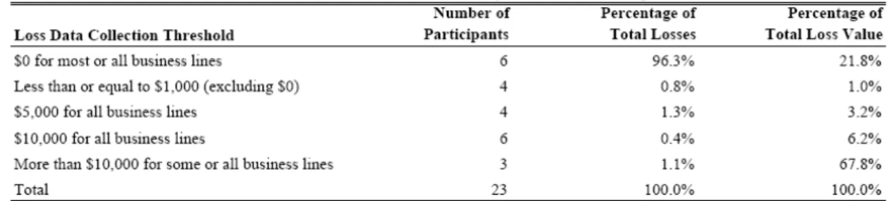
To evaluate impact of Basel II in minimum capital requirements, FED made a survey called QIS-4 (Quantitative Impact Study – 4) with the voluntary participation of institutions present in the U.S. A total of 27 institutions participated in two exercises proposed, but only 23 reported LDC data, presented in the published document with information summarize.
The collected loss data can be summarized in the following table by threshold and the number of institutions involved:
Table 1: Levels of the loss data collection threshold (published in Results of the 2004 Loss Data Collection Exercise for Operational Risk).
From the data presented we select Sample 1 to obtain meaningful results for loss frequency and loss severity. The sample only includes losses greater or equal to $10,000 and occurred during a time of period over which loss frequency appears to be stable. The data is build using three years of historical information related from 2002 to 2004. This study uses the data presents in Appendix 2 and 3, that allow to built the two crucial indicators to the proposal model: Average of Number of Events and Average Loss by Event (Appendix 4) , for both analytical dimensions: Event Type and Business Line. For each indicator are calculated simple average, weighted average and standard deviation. The values can be viewed in Appendix 5 and 6.
36 The following step is to perform Monte Carlo Simulations. First to event frequency (Poisson distribution) and then to Aggregated Losses using the five different distributions early presented. The results are reported in Appendix 7.
The final value for each business line or event type presents a significant range of amounts representing that the chosen distribution has influence in the result. Because the population is simulated using Monte Carlo is not possible to evaluate which distributions best fits to explain Operational Risk losses and has the best estimate for regulatory capital requirements.
4.2. ORX Report 2007
ORX Association is The Operational Riskdata eXchange Association is the world's leading operational risk loss data consortium for the financial industry. ORX was founded with the main goal of creating a sound platform for the secure and anonymised exchange of high-quality operational risk loss data.
ORX currently has 50 members and has over the past four years developed a database of 102,500 operational risk losses and can be very useful for its members as a credible data base for External Data to be used in their internal models of Operational Risk.
As the study presented before is only for US institutions, the ORX data capture realities majority from European markets but has also data from US and Canada. Notice that in terms of dimension the North America members’ revenues in average is the double of European members.
37 The data in this report can be summarized in the following table:
Table 2: High level Summary of ORX reported data
The data shows that the major losses took place in 2002 and 2003, but the number of events has increased over the years. The report also show that minor losses have higher frequency and higher losses have lower frequency, as expected in operational risk. With the data provided by the report about distribution of Loss Frequency and Loss Severity, similar to what is presented for FED, I calculate simple indicator to each Business Line and Event Type presented in Appendix 8.
The next steps are equal to FED and the results of Monte Carlo simulations and aggregated loss distributions estimated are presented in Appendix 9 and 10.
38 5. Conclusions
Basel II is a challenge for all institutions because it represents an opportunity to define and implement a model that allows managing Operational Risk and also to identify critical sources of Operational risk in their activities. This identification will give the chance to institutions to focus on improving risk management and being able to adjust regulatory capital to their risk profile.
This paper investigates the available methodologies to be applied to create an internal model to estimate regulatory capital using an Aggregated Loss methodology.
The data used in this paper has origin in two different reports, so they are aggregated and treated with different methodologies. This also allows using two different realities: US institutions in FED report and more European institutions in ORX report. Is not correct to simply compare the data but it is useful for testing the proposal model and simulating regulatory capital using different statistical distributions. These distributions are not symmetric. Gamma, Weibull and LogNormal are thin tailed distributions and Pareto is a “fat” tailed distribution, and because of their differences is possible to see different results, meaning that are some distributions that better fit some phenomenons than others, as the outputs graphs in the Appendix demonstrate.
For statistical treatment of frequency was used Poisson, that due to the distribution’s characteristics is the one that better fits to explain and estimate the frequency of operational risk events.
39 The CaR results obtained for both reports can be shown in the next figures divided by business line and event type:
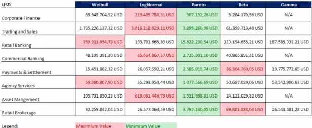
Figure 15: FED Final Output: Capital Requirement estimative by business line. The values are in US$.
Figure 16: FED Final Output: Capital Requirement estimative for each event type. The values are in US$.
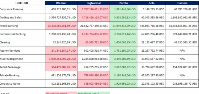
40 Figure 17: ORX Final Output: Capital Requirement estimative by business line. The values are in US$ (Exchange rate used in Appendix 1)
Figure 18: ORX Final Output: Capital Requirement estimative for each event type. The values are in US$. (Exchange rate used in Appendix 1)
From the statistical point of view Pareto’s estimative present the lowest values. This happens because Pareto’s does not depend on severity average and it uses the same parameters (shape and scale).
For ORX, Weibull and LogNormal Distributions return the higher estimative for CaR and for FED data Beta Distribution also presents higher values.
41 Due to the fact that I do not have real populations of events I can not make any statistical test to determine which one better describes expect behavior in any of the reports used. When looking to final results available in figures presented above, the major CaR appear in business lines and event type that in initial data had more frequency and severity as expected. It is in other business line or event type that the results show a higher variation between the minimum and maximum value estimates.
Is important to remember that ORX report has more years of historical and has been collected more recently, if we want to compare the results obtained.
This last fact may indicate that the data quality is better because institutions have developed in the past years more effective operational risk management policies and they have implemented also some procedures. It is also important to refer that their report is a voluntary decision as it is to be a member of ORX association.
The final values of the proposed model are higher than the initial ones as expected because this model has should be able to evaluate the capital needs to face expected and unexpected losses. The unexpected losses are the crucial values that regulatory capital should be able to cover when an operational risk loss happens, because the expected losses, institutions should be able to mitigate or for example to recover them in pricing or having contracted any type insurances.
The model’s principles establish in Basel II framework are very similar to VaR model, a concept introduced to measure market risk and used by all institutions. The important difference is that market risk losses are easy to track and report and operational risk losses are not, what transform the modeling process just the final step and focus the major concern is Loss Data Collection Process. For some opinions, these concerns are reflected in confidence level defined by Basel Committee of 99.90%, a conservative value that can be an indicator of some questions about historical data soundness and lack of knowledge for modeling process this type of factors.
The diversity of results obtain demonstrate that soundness information and their completeness is the challenge for all institutions, for building a strong internal model of Operational Risk that aims not just risk manage but also helps institutions to mitigate
42 risks and incentive them to adopt advanced approaches as a way to adjust regulatory capital to their own risk profile.
As this study was developed, Basel Committee published the 2008 LDCE for Operational Risk and an additional paper with the observed range of practice in key elements of Advanced Measurement Approaches. This exercise was the first international effort to collect information on all four data elements used in the AMA and with the bigger participation of institutions.
From the range of practice is important to retain the diversity of distributions used to modeling the severity of operational risk losses and the most representative are the same used in the model presented in this paper, as presented in the next figure:
Figure 19: Results presented by Basel Committee from the document “Observed range of practice in key elements of Advanced Measurement Approaches (AMA)”
The above figure show the values published regarding the application of one single distribution model for all data because is the same approach proposed in this paper. In this report of Basel Committee there are available data about other models used in practice.
This is important to support the model developed in this paper because the institutions are using real and detailed information and the majority is using approaches similar to the ones I proposed.
43 The main conclusion of this paper is that is crucial to consider all four elements to build a soundness model to estimate regulatory capital with internal models and information quality is the critical factor of success. Institutions should have in mind that is not enough to obtain a good fit based on statistical measures, but also that the model developed should be suitable for their reality.
44 6. References
(1) Maximum Likelihood from Incomplete Data via the EM Algorithm - A. P. Dempster, N. M. Laird and D. B. Rubin Journal of the Royal Statistical Society. Series
B (Methodological), Vol. 39, No. 1 (1977), pp. 1-38 (article consists of 38 pages)
(2) The EM Algorithm and Extensions, 2E
Series: Wiley Series in Probability and Statistics - Published Online: 30 Apr 2007 Author(s): Geoffrey J. McLachlan, Thriyambakam Krishnan
45 7. Bibliography
International Convergence of Capital Measurement and Capital Standards (November 2005), Basel Committee on Banking Supervision (BIS)
Operational risk management practices: Feedback from a thematic review (February 2005), Financial Services Authority
Operational Risk in Banks: an analysis of empirical data from an Australian Bank (September 2007), Institute of Actuaries of Australia
ORX Operational Risk Report (2007), ORX Association
Results of the 2004 Loss Data Collection Exercise for Operational Risk (May 12, 2005), Federal Reserve System Office of the Comptroller of the Currency Office of Thrift Supervision Federal Deposit Insurance Corporation
Results of the 2007 Operational Risk Data Collection Exercise (August 10, 2007), Planning and Coordination Bureau, Financial Service Agency Financial Systems and Bank Examination Department, Bank of Japan
Sound Practices for the Management and Supervision of Operational Risk (February 2003), Basel Committee on Banking Supervision (BIS)
The 2002 Loss Data Collection Exercise for Operational Risk: Summary of the Data Collected (March 2003), Basel Committee on Banking Supervision (BIS)
The Quantitative Impact Study for Operational Risk: Overview of Individual Loss Data and Lessons Learned (January 2002), Basel Committee on Banking Supervision (BIS)
Results from the 2008 Loss Data Collection Exercise for Operational Risk (July 2009), Basel Committee on Banking Supervision (BIS)
46 Observed range of practice in key elements of AMA (July 2009), Basel Committee on Banking Supervision (BIS)
Bühlmann, Hans; Shevchenko, Pavel V. & Wüthrich, Mario V. (February 19, 2007), A “Toy” Model for Operational Risk Quantification using Credibility Theory
Dempster, A.P.; Laird, N. M. & Rubin, D. B. (1977), Maximum Likelihood from Incomplete Data via the EM Algorithm published in Journal of the Royal Statistical
Society. Series B (Methodological), Vol. 39, No. 1
Haugh, Martin (2004), The Monte Carlo Framework, Examples from Finance and Generating Correlated Random Variables (IEOR E4703 – Fall 2004)
Jobst, Andreas A. (2007), Operational Risk – The Sting is Still in the Tail But the Poison Depends on the Dose (Working Paper version February 24, 2007), published in Journal of Operational Risk Vol. 2, No. 2 (Summer)
Jobst, Andreas A. (February 7, 2007), Constraints of Operational Risk Measurement and The Treatment of Operational Risk under the New Basel Framework, Working Paper
Leippold, Markus & Vanin, Paolo (November 3, 2003), The Quantification of Operational Risk
Laviada, Ana Fernández; García, Francisco Javier Martínez & Rodríguez, Francisco Somohano (August 2005), Operational risk management under Basel II: the case of the Spanish financial services – published in European Finance Association - 32nd Annual Meeting
McLachlan, Geoffrey J. & Krishnan, Thriyambakam (Second edition 2008), The EM Algorithm and Extensions
Valle, Luciana Dalla & Giudici, Paolo (2008) Bayesian Copulae distributions, with application to Operational Risk
47 Web Sites:
Bank for International Settlements, www.bis.org
ORX Association, www.orx.org
Gloria Mundi, www.gloriamundi.org
SAS Software, www.sas.com
Federal Reserve, www.federalreserve.gov
Scholar Google, http://scholar.google.pt/
48
Appendix
Appendix 1 Summary of Exchange Rates used in calculations EUR/USD
49 Appendix 2 FED LDCE DATA
Table A: Data Used in this document Source: LDCE 2004 – FED (Number of Losses, Annualized By Business Line and Event Type Sample 1: losses ≥ $10,000 Occurring in Years When Data Capture Appears Stable
50 Appendix 3 FED LDCE DATA
Table B: Data Used in this document Source: LDCE 2004 – FED (Total Loss Amount ($US Millions), Annualized By Business Line and Event Type Sample 1: losses ≥ $10,000 Occurring in Years When Data Capture Appears Stable
51 Appendix 4 FED LDCE DATA
Table C: Data Output for Average Loss by event of Operational Risk using information presented in Appendix 2 and 3. The values are in $US Millions
52 Appendix 5- 2004 FED LDCE
Table E: Descriptive Statistics for the Average Loss by business line and event type using Appendix 2 and Appendix 3 data
53 Appendix 6: ORX Report 2007: Original Data
54 Appendix 7: ORX Report 2007 – Descriptive Statistics
Table G: Descriptive Statistics for the Average Loss by business line and event type using ORX data. The values are in Euros Thousands
55 Appendix 8: 2007 ORX Report – Results produced by the model (representative graphs for each distribution by Business Line
56 Exhibit 8.2: Asset Management
57 Exhibit 8.3: Clearing
58 Exhibit 8.4: Commercial Banking
59 Exhibit 8.5: Corporate Finance
60 Exhibit 8.6: Corporate Items
61 Exhibit 8.7: Private Banking
62 Exhibit 8.8: Retail Brokerage
63 Exhibit 8.9: Trading & Sales
64 Exhibit 8.10: Retail Banking
65 Appendix 9: 2007 ORX Report – Results produced by the model (representative graphs for each distribution by Event Type
Exhibit 9.1: Clients, Products and Business Practices
66 Exhibit 9.2: Disasters and Public Safety
67 Exhibit 9.3: Employment Practices and workplace Safety
68 Exhibit 9.4: Technology and Infrastructures Failures
69 Exhibit 9.5: Execution, Delivery and Process Management
70 Exhibit 9.6: External Fraud
71 Exhibit 9.7: Internal Fraud
72 Appendix 10 2007 FED Results produced by the model (representative graphs for each distribution by Business Line
Exhibit10.1 Agency Services:
73 Exhibit 10.2 Asset management
74 Exhibit 10.3 Commercial Banking
75 Exhibit 10.4 Corporate Finance
76 Exhibit 10.5 Payments & Settlements
77 Exhibit 10.6 Retail Banking
78 Exhibit 10.7 Retail Brockerage
79 Exhibit 10.6 Trading & Sales
80 Appendix 11 2007 FED Results produced by the model (representative graphs for each distribution by Event Type
Exhibit 11.1 Business Distribution