ABSTRACT: Soil sampling is an important stage of digital soil mapping. The objective of this study was to characterize the spatial design of soil sampling using soil apparent electrical conductivity (ECa) and its optimized spatial sampling. For the characterization, it was used the Spatial Simulated Annealing (SSA) technique, incorporated on the software SANOS 0.1, and the method of response surface sampling design on the software ESAP 2.35. The ECa was measured at 1,887 points in an area of 6 ha located in the northwestern region of Spain. The EM38-DD equipment (Geonics Limited 2005) was used at 2 depths: vertical
Soil And PlAnT nuTRiTion -
Article
Spatial soil sampling design using apparent
soil electrical conductivity measurements
Glécio Machado Siqueira1*, Jorge Dafonte Dafonte2, Antonio Paz González3, Eva Vidal Vázquez3, Monteserrat Valcarcel Armesto2, Osvaldo Guedes Filho41. Universidade Federal do Maranhão - Departamento de Geociências - São Luís (MA), Brazil.
2. Universidad de Santiago de Compostela - Departamento de Ingeniería Agroflorestal - Lugo (Galicia), Spain. 3. Universidade da Coruña - Facultad de Ciencias - La Coruña (Galicia), Spain.
4. Universidade Federal do Paraná - Jandaia do Sul (PR), Brazil.
*Corresponding author: gleciosiqueira@hotmail.com
Received: Sept. 17, 2015 – Accepted: Mar. 6, 2016
dipole (1.5 m effective measurement depth) and horizontal dipole (0.75 m effective measurement depth). Semivariogram showed trend for ECa in vertical dipole (ECa-V) and ECa in horizontal dipole (ECa-H). Software SANOS 0.1 and ESAP 2.35 were used to obtain the 40-point sampling scheme, using the 2 schemes (SANOS and ESAP). ECa-V estimation values at the 1,887 points were calculated with residual ordinary kriging. The sampling scheme obtained from ESAP was better than with SANOS.
inTRoduCTion
The soil sampling is an important stage of digital soil mapping (DSM). In DSM the principal idea is that soil properties have some sort of correlation with other environmental variables. These variables are known as secondary information in a regular grid or densely sampling, i.e. digital elevation models, geological maps, remote sensing images, apparent soil electrical conductivity
(ECa) or resistivity (McBratney et al. 2003).
ECa, measured by contact or by electromagnetic
induction, is directly related with other physical and chemical soil properties. There are some factors that may
affect the ECa: soil moisture, pore size distribution, salt
content, particle size distribution, cation exchange capacity (CEC), clay mineral composition, pore geometry and tortuosity, concentration of dissolved electrolytes in soil water, amount and composition of colloids, and temperature of soil water (Sudduth et al. 2005; Kühn et al. 2008; Siqueira
et al. 2015a). Several authors have used ECa to improve the
estimation of other soil properties (McNeill 1980; Lesch et al. 2000; Schumann and Zaman 2003; Domsch and Giebel 2004; Sudduth et al. 2005; Amezketa 2007). Therefore, the use of
ECa measured by electromagnetic induction is an important
tool soil digital mapping, favoring the use of optimized sampling schemes.
Spatial sampling schemes are used to determine the sample location describing the spatial variability of determined variables. Besides the grid configuration, sampling density and distance are important factors for accurate spatial predictions (Minasny and McBratney 2007). Sampling schemes can be optimized using geostatistical methods as described by van Groenigen et al. (1999) as well as Diggle and Lophaven (2006). One of the main criticisms of geostatistical approach is the necessity of prior knowledge of attributed semivariogram. Other methods are based on geometric criteria, without semivariogram estimation, as it was proposed by Royle and Nychka (1998), or on statistical criteria, as the method proposed
by Lesch et al. (1995), who used ECa data based on a
multiple regression model to determine the samples’ number and location.
Two complex mathematical models have been widely used to specify the optimum sampling schemes of soil and plant: SANOS 0.1 (van Groenigen et al. 1999) and Electrical Conductivity or Salinity, Sampling, Assessment
and Prediction (ESAP) 2.35 software (Lesch et al. 2000). However, there is no study evaluating the accuracy of these methods in respect to the original data. SANOS 0.1 software has an open system that allows to determine any number of samples for a previously studied area, while the ESAP 2.35 software has limitations regarding the number of points to be optimized and it was developed specifically for soil electrical conductivity and salinity data.
Other authors have used the ESAP software to optimize the use of satellite images (Hunsaker et al. 2009). Ferreyra et al. (2002) used the SANOS software to reduce the number of soil moisture samples having as secondary tool for decision making the scaled semivariogram. Siqueira et al. (2015b) studied different sampling schemes and soil water contents. They observed that the choice of sampling scheme influenced the results, particularly in relation to small number of samples, preventing the use of geostatistical techniques and precision agriculture.
The objective of this study was to characterize the spatial
design of soil sampling, using ECa and its optimized spatial
sampling. For that, the Spatial Simulated Annealing (SSA) technique was used incorporated on SANOS 0.1 software, as well as the method of sampling design by response surface using ESAP 2.35 software.
MATERiAl And METHodS
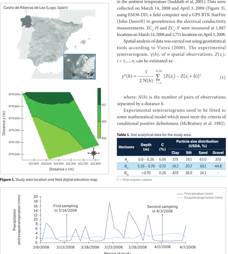
The study area (6 ha) is located at Castro de Ribeiras de Lea, Lugo, Spain. The geographical coordinates are
43°09′49″N and 7°29′47″W, with average elevation of
410 m and average slope of 2% (Figure 1). The mean annual temperature is 11.2 °C and the mean annual rainfall is 930 mm (data: 1961 – 1990) (Paz González et al. 1996).
Daily rainfall (mm) and crop reference evapotranspiration (mm) are shown in Figure 2. The soil area is classified according to FAO-ISRIC (1994) as Cambisol, with parent material of sediments from tertiary and quaternary periods (Paz González et al. 1997). Table 1 shows the particle size distribution and organic carbon. The organic matter
content is higher in the horizon Ap compared to the other
soil horizons. Soil texture (size < 2 mm) is sandy-loam
in the horizon Ap, loam-clay-sandy in the horizon Bw and
clay in the horizon Btg.
The ECa (mS∙m
−1) was measured with an induction
The equipment consists of 2-unit measurements: one in a
horizontal dipole (ECa-H), to provide an effective measurement
depth of approximately 0.75 m, and another in a vertical dipole
(ECa-V), with an effective measurement depth of approximately
1.5 m (McNeill 1980), which cover the complete root volume
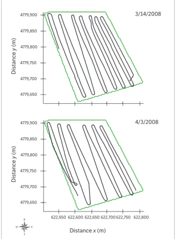
of a plant (Domsch and Giebel 2004). The principle of the EM38-DD device requires the instrument to be calibrated a new at each location and before each measurement (Geonics Limited 2005). The instrument must also be calibrated a new if the instrument’s temperature changes because of alterations in the ambient temperature (Sudduth et al. 2001). Data were collected on March 14, 2008 and April 3, 2008 (Figure 3), using EM38-DD, a field computer and a GPS RTK StarFire
(John Deere®) to georeference the electrical conductivity
measurements. ECa-H and ECa-V were measured at 1,887
locations on March 14, 2008 and 1,751 locations on April 3, 2008. Spatial analysis of data was carried out using geostatistical tools according to Vieira (2000). The experimental
semivariogram, γ(h), of n spatial observations, Z(xi),
i =1,..., n, can be estimated as:
622,550 622,600 622,650 622,700 622,750 622,800
Distance x (m)
Distance
y
(m)
4779,650 4779,700 4779,750 4779,800 4779,850 4779,900
406 409 412
Castro de Ribeiras de Lea (Lugo, Spain)
Figure 1. Study area location and field digital elevation map.
Figure 2. Precipitation and potential crop reference evapotranspiration in the period of study.
4/2/2008 First sampling
in 3/14/2008
Second sampling in 4/3/2008
Precipitation
and evapotranspiration (mm)
Precipitation (mm) Evapotranspiration (mm)
20 18 16 14 12 10 8 6 4 2 0
3/8/2008 3/13/2008 3/18/2008 3/23/2008
Period of study
3/28/2008 4/7/2008
Horizons depth (m)
C (%)
Particle size distribution (uSdA, %)
Clay Silt Sand Gravel
Ap 0.0 – 0.35 5.05 17.5 19.1 63.0 37.0
Bw 0.35 – 0.70 0.72 19.2 20.7 59.1 44.8
Btg +0.70 0.26 47.9 28.0 24.1
-C = Total organic carbon.
Table 1. Soil analytical data for the study area.
γ*(h) = [Z(xi) – Z(xi + h)]2
∑
1
2 N(h) i = 1
N (h)
where: N(h) is the number of pairs of observations
separated by a distance h.
Amongst all the variety of models which satisfy that condition, the fitting parameters that describe them are the nugget effect, C0, the sill, C0 + C1 (where C1 is the structured variance coefficient to be defined later), and the range of spatial
dependence a.
When the semivariogram of any particular variable does not stabilize at constant value for the sill, it is evident that the sill does not exist. Therefore, the stationarity of the mean may not be guaranteed because the variable increases in an unlimited way in some direction. In this situation, it is necessary to remove the trend before any geostatistical application based on the intrinsic hypothesis (Vieira 2000). One possible way to detrend the data is using a trend surface fitted to data through minimized squared deviations of the difference between the surface and the original data, producing a new residual variable
(Vieira 2000). In this study, ECa (mS∙m
−1) showed some
trend that was best fitted to a parabolic surface, Ztrend,
using the following equation:
where: A0, A1, A2, A3, A4 and A5 are the fitting parameters.
The residual variable, Zres, can be obtained by subtracting
the estimated trend surface from the original values for each point:
3/14/2008
4/3/2008
622,550 622,600 622,650 622,700 622,750 622,800
Distance x (m)
Distance
y
(m)
4779,650 4779,700 4779,750 4779,800 4779,850 4779,900
Distance
y
(m)
4779,650 4779,700 4779,750 4779,800 4779,850 4779,900
Figure 3. Sampling scheme of soil apparent electrical conductivity.
Ztrend = A0 + A1x + A2 y + A3x2 + A 4 y
2 + A
5xy Pc (Si → Si+1) = 1
Zres(x,y) = Z(x,y) − Ztrend(x,y)
In Equation 3, the variable Zres is subsequently tested
for the existence of a defined sill in the semivariogram. The kriging estimation is done on the residual values to which the estimated surface is added after the estimation is done.
As the semivariograms for the original data showed a very strong trend, violating the intrinsic hypothesis of geostatistics (Journel and Huijbregts 1978), parabolic trend surface equations were fitted to the data and subtracted from them. The residuals generated by the difference between originals and trend surface produced semivariograms that showed a very well-defined sill, and, for this reason, the residuals were used in the remaining analysis; the semivariogram model was fitted using the cross validation by means of the software Gstat (Pebesma 1992).
It was used the SANOS 0.1 software (van Groenigen et al. 1999) to locate the new sampling location points
of ECa, with the criteria of optimization sample and the
mitigation of ordinary kriging variance average in the study area, through a spatial simulation algorithm (SSA) that uses the fitting parameters of variable semivariograms. The parameters of the residuals in semivariogram models
(ECa-V and ECa-H) were determined at 40 locations where
ECa was measured. SSA is a continuous version of the
discrete Simulated Annealing (SA) optimization method (Aarts and Korst 1989). The insensitivity of the algorithm to local extremes makes it very suitable for constrained optimization of spatial sampling schemes in the presence of complex pre-information. Consider the collection of
possible sampling schemes consisting of n observations,
Sn, with a so-called fitness function φ(·):Sn → View the
MathML source+ to be minimized. Optimization starts
with a random scheme S0 ∈ Sn. It then involves a sequence of
proposed random perturbations Si+ 1 of S0 that have
a probability Pc(Si → Si+1) of being accepted. This transition
probability is defined in the Metropolis criteria:
(2)
(3)
where: c denotes the positive control parameter, which is lowered as optimization progresses.
If Si+1 is accepted, it serves as a starting point for a next
scheme Si+2,and the process continues in a similar way
(Aarts and Korst 1989). In SSA, random perturbations
of the sampling scheme Si consist of transformations of
randomly-chosen observations over a vector with random length and random direction. We will consider a vector
δin of n elements. At each step an element is selected at
random, and it is assigned a random value. All other values are equal to 0. This vector has the following
property: |δin| → 0 when i → ∞. SSA can include earlier
observations into the optimization by treating them as an integral but fixed part of the sampling scheme, i.e.
with corresponding δin values set equal to 0 for all i.
Boundaries of the region and inaccessible sub-regions can be taken from a GIS file.
Until the present moment, several optimization criteria have been translated into a fitness function and applied in SSA. Two of those are important in this study: (a) MMSD-criterion, which aims a spreading of the observations over the entire research area by minimizing the distance between an arbitrarily chosen point and its nearest observation; (b) WM-criterion, which is taken from the literature and optimizes the fit of the realized distribution of point pairs for the experimental variogram to a pre-defined, ideal distribution (Russo 1984; Warrick and Myers 1987; Russo and Jury 1988). The desired distribution can be based upon expert judgment, allowing the user to give special attention to certain aspects of the variogram (for instance, the nugget). The minimization function is a simple sum of squares of the deviation between the desired distribution ζ* and the realized distribution ζS.
The ESAP 2.35 software (Lesch et al. 2000) was also used to determine the optimum position of the 40 sample points. For this, it was used the computational tool ESAP-RSSD (Response Surface Sampling Design) that uses a multiple linear regression model minimizing the chances of autocorrelation space between the surface of different models of response generated by the algorithm,
as reported by Lesch et al. (1995) and Fitzgerald et al. (2006). In this method, optimized sampling scheme process
begins with log-transformation (ln) of ECa measurements
in vertical dipole (lnECa-V) and in horizontal dipole
(lnECa-H), obtaining a variable with combined trend
surface, considering the original location (x,y) (Lesch
et al. 2000). Later, ECa-V = z1 and ECa-H = z2 are correlated with location coordinates of presumed surface. It is possible to minimize the values obtained in the prediction and estimate values that represent the different reply surfaces for each new configuration:
where: x and y are the geographic coordinates;
z1= b1[lnECa-V − average(lnECa-V)] + b2[lnECa-H −
average(lnECa-H)]; z2= b3[lnECa-V − average(lnECa-V)]
+ b4[lnECa-H − average(lnECa-H)]; b0, b1, b2, b3 and b4
are the estimated parameters; u = (x − min[x])/k;
v = (y − min[y])/k; k is the maximum value of (max[x] − min[x])
or (max[y] − min[y]).
To choose the best location of ECa for the new sampling
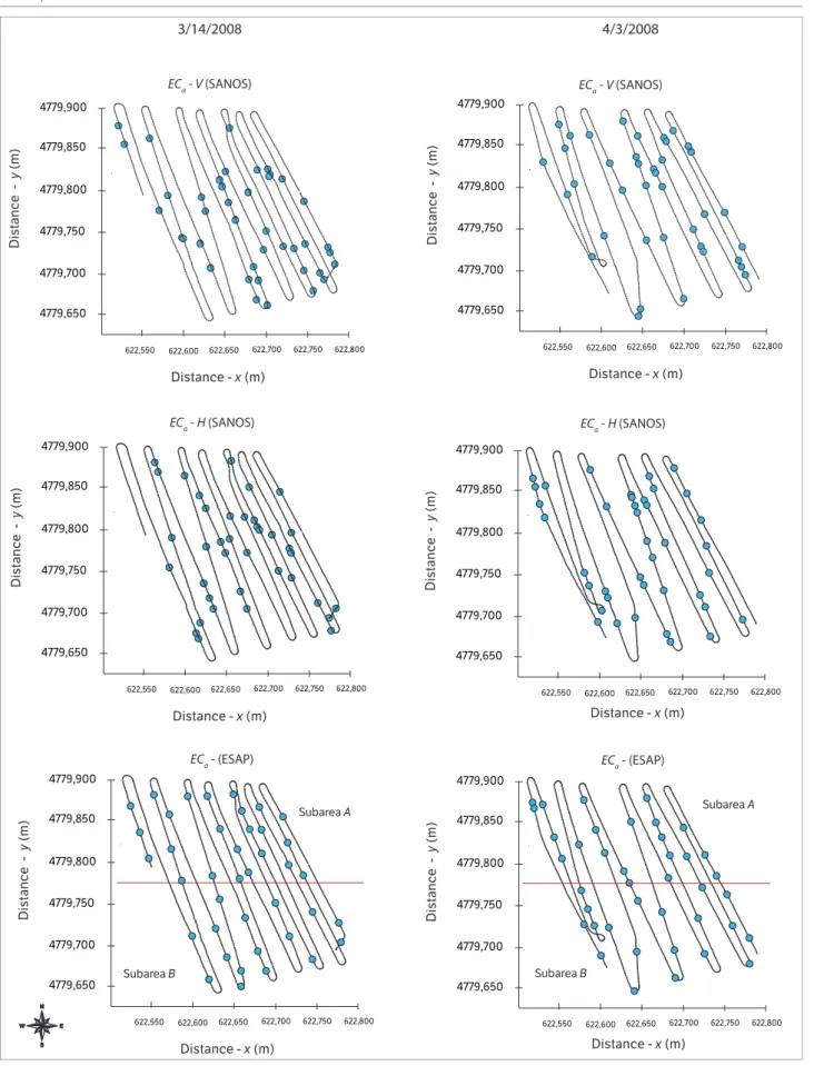
model, all the parameters have to be significantly different from zero (p > 0.05) and with the minimum predicted residual sum of squares. The spatial independence of residues was examined using the residual autocorrelation test of Moran (Brandsma and Ketellapper 1979; Lesch et al. 1995). ESAP-RSSD software lets the determination of 6; 12 and 20 points of optimized sampling scheme. Our
study area was divided into 2 subareas (A and B). In each
subarea the ESAP-RSSD software was used to determine the sampling scheme of 20 locations and to obtain, with the 2 subareas, 40 locations of sampling scheme for all the field. The SANOS 0.1 software does not have any restriction about the location number of sampling scheme in the field.
Using the sampling points chosen by SANOS and
ESAP, and the measured values of ECa-V and ECa-H at
those points, the semivariogram was performed using the residual values. The residual is the difference between the regionalized variable and the trend. The residual ordinary kriging was used to estimate residuals of 1,887 and 1,751
values of ECa-V measured with the EM38-DD (ECa-Vmea)
with the Gstat software (Pebesma 1992). After the residual estimation, it was added to the trend estimation for each
point, obtaining an estimate of ECa-V (ECa-Vest) from the 40
if ϕ (Si+1) ≤ ϕ (Si)
if ϕ (Si+1) > ϕ (Si)
ln (ECa) = b0 + b1(z1) + b2(z2) + b3(u) + b4(v)
Pc (Si → Si+1) = exp [ ϕ (Si) – ϕ (Si+1)]/c (4)
sampling points chosen by SANOS and ESAP. To estimate the performance of the 2 sampling schemes, the sum of squared errors (SSE) obtained with SANOS and ESAP was used in the Equation 7:
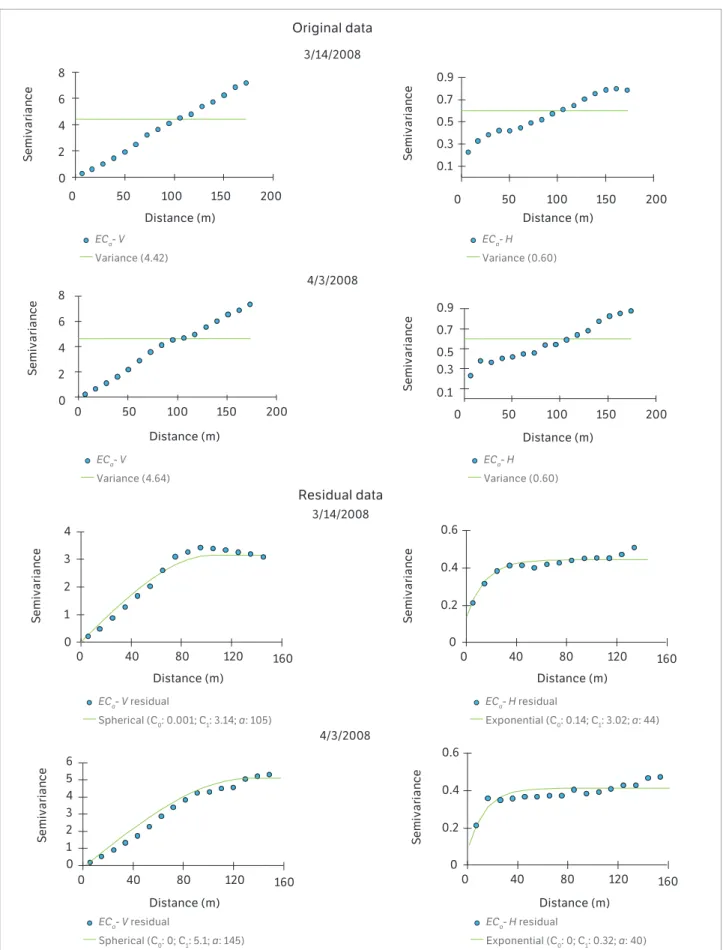
semivariograms in both dates have had the same model, the spatial variability pattern was not the same. This difference is most important at the initial part of the semivariogram that represents the spatial variability at short distances.
The fitted parameters of semivariogram showed low spatial discontinuity between dates; it means that the
nugget effect values (C0) were low for all data sets (Figure 4).
Range values (a) varied from 105 m for ECa-V in March
14, 2008 to 145 m for April 3, 2008. ECa-H data presented a
low value of range for the second measurement date (40 m) in relation to the first one (40 m). The difference between
ECa-V and ECa-H range values is mainly caused by the
greater measurement volume in vertical dipole. This fact is responsible for a lower spatial discontinuity.
Sample scheme optimization using ESAP 2.35 and SANOS 0.1 software showed a different sample scheme for the 2 methods and for the 2 measurement dates (Figure 5). In SANOS the variation in semivariogram parameter values resulted in different sampling schemes. The SANOS software lets the choice of location number in the other side the ESAP software the user can only use 6; 12 or 20 sample locations. Therefore, if the user wants to use a greater location number in field, it is necessary to subdivide the fields in several subfields.
There is no agreement about the kriging variance minimization as measurement of local uncertainty. Goovaerts (1997) showed that kriging variance is mainly influenced by the spatial configuration of data. ESAP software uses the 2 measurements of soil apparent
electrical conductivity (ECa-V and ECa-H) and their
locations (Lesch et al. 2000). ESAP software has a simple use, because it is not necessary to know the variable semivariograms previously to sampling location optimization.
Experimental semivariograms were calculated using the
measured ECa in the optimized sampling points (Figure 6).
These semivariograms showed trends, which were removed, and residual semivariograms were obtained.
RESulTS And diSCuSSion
The data sets presented a log-normal distribution (Table 2).
ECa-V showed the greatest variance values in both times,
because the soil volume measurements in vertical dipole is greater than in the horizontal. In this way, the major differences are mainly caused by intrinsic soil factors as clay content, water content and dissolved cations in soil solution (Rhoades et al. 1976; Nadler and Frenkel 1980; McNeill 1980). The values of standard deviation (SD) and coefficient of variation (CV) followed the same pattern.
The ECa data showed trend, i.e. the semivariance
values increase when distance increases (Figure 4). The
observed trend for all ECa data was quadratic. In this case,
the presence of trend is related to the area topography with a 2% slope (Figure 1), which contributes to water flow in downhill direction and causes the greatest values of water content in the lowest area in the field. According to Kuzyakova et al. (1997), soil topography is one of the main factors that affect the soil spatial variability; they described that landscape shape (concave, convex or lineal) has different spatial variability caused mainly by the different water flow in the soil.
The residual semivariograms of ECa-V were fitted to spherical
model; meanwhile, ECa-H was fitted to the exponential one
(Figure 4). Several authors have described that spherical model is the most common for soil and plant properties (McBratney and Webster 1986; Cambardella et al. 1994; Carvalho et al. 2002;
Siqueira et al. 2008). The ECa-V semivariograms presented
the same spatial variability pattern. Although the ECa-H
date Attribute
(mS∙m−1) Mean Variance
Standard deviation
Coefficient of
variation (%) Skewness Kurtosis
03/14/2008 ECa-V 10.48 4.42 2.10 20.07 0.527 0.124
ECa-H 14.10 0.60 0.77 5.53 0.065 1.810
04/03/2008 ECa-V 14.04 4.64 2.15 15.34 0.662 0.083
ECa-H 14.59 0.60 0.77 5.32 0.160 10.514
Table 2. Statistical parameters of soil apparent electrical conductivity in vertical and horizontal dipoles.
0 2 4 6 8
0 2 4 6 8
0 50 100 150 200
0 50 100 150 200
S
e
m
iv
a
ri
a
n
c
e
S
e
m
iv
a
ri
a
n
c
e
Distance (m) Distance (m)
S
e
m
iv
a
ri
a
n
c
e
Distance (m)
0 1 2 3 4
0 40 80 120 160
0 40 80 120 160
EC
a- V residual
Spherical (C0: 0; C1: 5.1; a: 145)
0 40 80 120 160
0 0.2 0.4 0.6
0 40 80 120 160
0 0.2 0.4 0.6
0 1 2 3 4 5 6
3/14/2008
4/3/2008 Original data
0 50 100 150 200
Distance (m)
0 50 100 150 200
0.1 0.3 0.5 0.7 0.9
S
e
m
iv
a
ri
a
n
c
e
S
e
m
iv
a
ri
a
n
c
e
S
e
m
iv
a
ri
a
n
c
e
Distance (m) Distance (m)
S
e
m
iv
a
ri
a
n
c
e
Distance (m)
3/14/2008
4/3/2008 Residual data
Distance (m)
S
e
m
iv
a
ri
a
n
c
e
0.1 0.3 0.5 0.7 0.9
EC
a- V residual
Spherical (C0: 0.001; C1: 3.14; a: 105)
EC
a- H residual
Exponential (C0: 0.14; C1: 3.02; a: 44)
EC a- V Variance (4.64)
EC a- H Variance (0.60) EC
a- V Variance (4.42)
EC a- H Variance (0.60)
EC
a- H residual
Exponential (C0: 0; C1: 0.32; a: 40)
622550 622600 622650 622700 622750 622800 Distancia X (m)
4779650 4779700 4779750 4779800 4779850 4779900
Dista
nce Y
(
m
)
622550 622600 622650 622700 622750 622800
Distance X (m) 4779650
4779700 4779750 4779800 4779850 4779900
D
is
ta
n
c
e
Y
(
m
)
622550 622600 622650 622700 622750 622800
Distance X (m) 4779650
4779700 4779750 4779800 4779850 4779900
Dista
nce
Y
(
m
)
622550 622600 622650 622700 622750 622800
Distance X (m) 4779650
4779700 4779750 4779800 4779850 4779900
Di
s
ta
n
ce Y
(
m
)
622550 622600 622650 622700 622750 622800
Distance X (m) 4779650
4779700 4779750 4779800 4779850 4779900
Di
s
tan
ce Y
(
m
)
622550 622600 622650 622700 622750 622800
Distance X (m) 4779650
4779700 4779750 4779800 4779850 4779900
Distan
ce Y
(
m
)
622,550 622,600 622,650 622,700 622,750 622,800 4779,650
4779,700 4779,750 4779,800 4779,850 4779,900
Distance -
y
(m)
Distance - x (m) 622,550 622,600 622,650 622,700 622,750 622,800
4779,650 4779,700 4779,750 4779,800 4779,850 4779,900
Distance -
y
(m)
Distance - x (m)
622,550 622,600 622,650 622,700 622,750 622,800 4779,650
4779,700 4779,750 4779,800 4779,850 4779,900
Distance -
y
(m)
Distance - x (m) 622,550 622,600 622,650 622,700 622,750 622,800
4779,650 4779,700 4779,750 4779,800 4779,850 4779,900
Distance -
y
(m)
Distance - x (m)
622,550 622,600 622,650 622,700 622,750 622,800 4779,650
4779,700 4779,750 4779,800 4779,850 4779,900
Distance -
y
(m)
Distance - x (m) 622,550 622,600 622,650 622,700 622,750 622,800
4779,650 4779,700 4779,750 4779,800 4779,850 4779,900
Distance -
y
(m)
Distance - x (m) 3/14/2008
ECa - H (SANOS)
ECa - V (SANOS)
ECa - (ESAP)
ECa - H (SANOS)
ECa - V (SANOS)
ECa - (ESAP) 4/3/2008
Subarea A Subarea A
Subarea B Subarea B
0 0.5 1 1.5 2 2.5 3 3.5 4 4.5 5
0 50 100 150 200
ECa -V Va ria nce (3.23)
0 0.2 0.4 0.6 0.8 1 1.2 1.4
0 50 100 150 200
ECa -H Va ria nce (0.77)
0 1 2 3 4 5 6 7 8 9
0 50 100 150 200
ECa -V Va ria nce (5.04)
0 0.2 0.4 0.6 0.8 1 1.2
0 50 100 150 200
ECa -H Va ria nce (0.71)
0 0.2 0.4 0.6 0.8 1 1.2 1.4 1.6 1.8
0 50 100 150 200
ECa -V Va ria nce (0.78)
0 1 2 3 4 5 6 7 8
0 50 100 150 200
ECa -H Va ria nce (3.95)
0 1 2 3 4 5 6 7 8
0 50 100 150 200
0 0.1 0.2 0.3 0.4 0.5 0.6 0.7 0.8 0.9 1
0 50 100 150 200
ECa -H Va ria nce (0.65)
0 2 1 3 4 5 1 3 5 7 9
0 50 100 150 200
0 50 100 150 200
S e m iv a ri a n c e S e m iv a ri a n c e
Distance (m) Distance (m)
S e m iv a ri a n c e Distance (m)
3/14/2008 – SANOS
3/14/2008 – ESAP
Original data for optimized sampling points
0 50 100 150 200
Distance (m)
0 50 100 150 200
0.2 0 0.6 0.4 0.8 1.2 1 1.4 S e m iv a ri a n c e
4/3/2008 – SANOS
4/3/2008 – ESAP
0.2 0.6 0.4 0.8 1 1.2 EC a- V
Variance (5.04)
EC a- H
Variance (0.71)
ECa- V
Variance (3.23)
ECa- H
Variance (0.77) 1 1.4 0.6 0.2 1.8 0 2 4 6 8
0 50 100 150 200
0 50 100 150 200
S e m iv a ri a n c e S e m iv a ri a n c e
Distance (m) Distance (m)
S e m iv a ri a n c e Distance (m)
0 50 100 150 200
Distance (m)
0 50 100 150 200
8 6 4 2 0 S e m iv a ri a n c e 0.1 0.3 0.5 0.7 0.9 EC a- V
Variance (5.44)
EC a- H
Variance (0.65)
ECa- V
Variance (0.78)
ECa- H
Variance (3.95)
Figure 6. Experimental and fitted model semivariograms for optimized sampling points.
Figure 6. Experimental and fitted model semivariograms for optimized sampling points. 0 0.1 0.2 0.3 0.4 0.5 0.6
0 20 40 60 80 100 120 140 160
0 0.5 1 1.5 2 2.5 3 3.5 4 4.5 5
0 20 40 60 80 100 120 140 160
0 0.1 0.2 0.3 0.4 0.5 0.6 0.7 0.8
0 20 40 60 80 100 120 140 160
0 0.5 1 1.5 2 2.5 3 3.5
0 20 40 60 80 100 120 140 160
0 0.1 0.2 0.3 0.4 0.5 0.6 0.7
0 20 40 60 80 100 120 140 160
0 0.5 1 1.5 2 2.5 3 3.5 4
0 20 40 60 80 100 120 140 160
0 0.1 0.2 0.3 0.4 0.5 0.6 0.7
0 20 40 60 80 100 120 140 160
0 0.5 1 1.5 2 2.5 3
0 20 40 60 80 100 120 140 160
0 1 2 3 0 1 2 3 4
0 40 80 120 160
S e m iv a ri a n c e S e m iv a ri a n c e
Distance (m) Distance (m)
S e m iv a ri a n c e Distance (m)
3/14/2008 – SANOS
3/14/2008 – ESAP
Residual data for optimized sampling points
Distance (m) 0.1 0.3 0.5 0.7 S e m iv a ri a n c e
4/3/2008 – SANOS
4/3/2008 – ESAP
0.1 0.3 0.5 0.7
EC
a- V residual (ESAP, Subarea A + B) Gaussian (C0: 0; C1: 3.6; a: 90)
EC
a- H residual (ESAP, Subarea A + B) Variance (4.39)
EC
a- V residual (SANOS) Spherical (C0: 0; C1: 2.6; a: 105)
EC
a- H residual (SANOS) Variance (0.48) 1.5 2.5 0.5 3.5 0 1 2 4 5 S e m iv a ri a n c e S e m iv a ri a n c e Distance (m) S e m iv a ri a n c e Distance (m) 3 Distance (m) 0.2 0.4 0.6 0.8 0 S e m iv a ri a n c e 0 0.2 0.4 0.6 EC
a- V residual (ESAP, Subarea A + B) Spherical (C0: 0; C1: 4.2; a: 120)
EC
a- H residual (ESAP, Subarea A + B) Exponencial
EC
a- V residual (SANOS) Spherical (C0: 0; C1: 2.8; a: 100)
EC
a- H residual (SANOS) Variance (0.5)
0 40 80 120 160
0 40 80 120 160
0 40 80 120 160
0 40 80 120 160
0 40 80 120 160
0 40 80 120 160
0 40 80 120 160
Residual semivariograms for the 40 optimized sampling locations by ESAP for the 2 dates were fitted to spherical model
(Figure 6). The ECa-H residual semivariograms did not
show spatial dependence in the studied scale for the first sampling date for the 2 used software (ESAP and SANOS).
For the second sampling date (April 3, 2008) the ECa-H
residual semivariogram showed spatial dependence for the sampling scheme obtained by ESAP software and nugget effect with SANOS software. This finding shows that it is not spatial dependence between samples, or separation distance between samples is greater than the minimum radius of spatial variability areas (Vieira 2000). Nugget
values (C0) were low for all variables that showed spatial
dependence. This fact indicates low variability of data.
Range values (a) increase 20 m for ECa-V residual from
the first to the second sampling date in the sampling scheme obtained with ESAP. Meanwhile the range values of data obtained with SANOS remained stable.
The ECaspatial variability maps (ECa-V and ECa-H) for
data measured in March 14, 2008 and April 3, 2008 showed a
similar spatial pattern. Lower values of ECa were found in the
northwestern area (Figure 7). ECa-H map was less smooth,
because the samples are spatially correlated in a shorter distance
than ECa-V, according to the range values (Figure 4). ECa-H
had distance correlation between samples of 40 m, and ECa-V
showed distance correlation around 105 – 145 m.
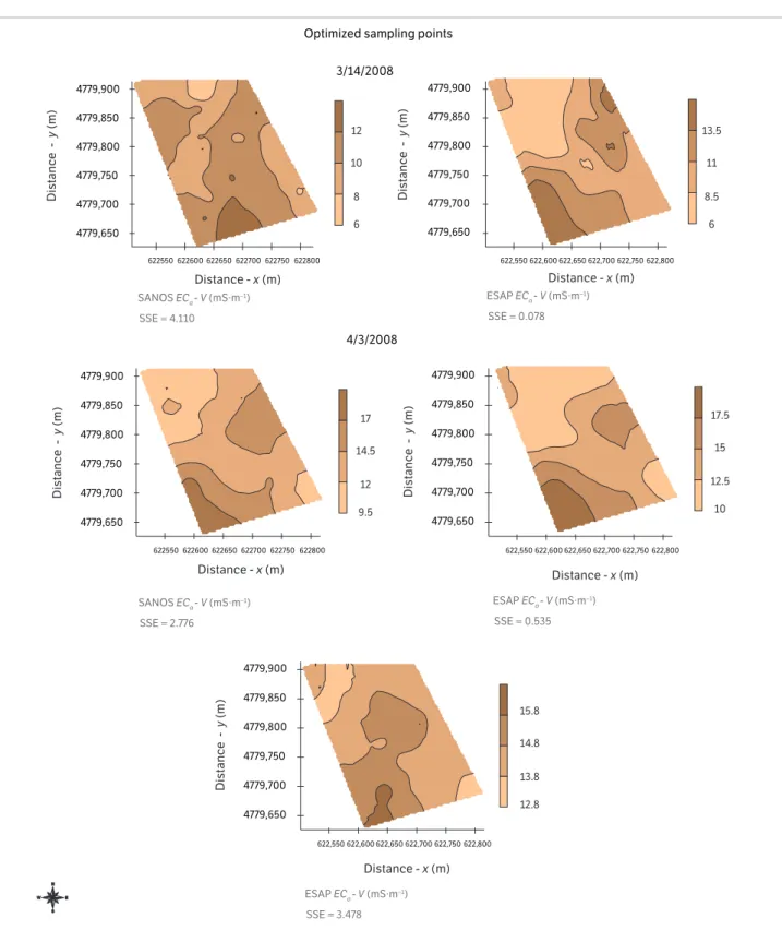
Spatial variability maps of ECa-V and ECa-H made
from the sampling schemes optimized by ESAP and SANOS (Figure 8) showed that maps obtained by ESAP were similar to the maps constructed using the measured values (Figure 7). This similarity is greater in the estimated
maps for ECa-V.
The values of ECa-V calculated by ordinary kriging in
the measurement locations using the data measured in these sampling schemes optimized by ESAP showed
low values of SSE (Figure 8). The value of SSE for ECa-H
in April 3, 2008 obtained with ESAP was greater. For this residual semivariogram the range value was low (65 m); this fact causes a smaller spatial variability area. The SSE values diminish from the first to the second sampling
Figure 7. Map of the estimated values obtained by ordinary kriging for original data.
Original data 3/14/2008
4/3/2008
4779,650 4779,700 4779,750 4779,800 4779,850 4779,900
6 9.5 13 16.5
9.5 11.5 13.5 15.5
622550 622600 622650 622700 622750 622800 4779,650
4779,700 4779,750 4779,800 4779,850 4779,900
10 13 16 19
622,550 622,600 622,650 622,700 622,750 622,800 622550 622600 622650 622700 622750 622800 622,550 622,600 622,650 622,700 622,750 622,800
8 11 14 17
Distance -
y
(m)
Distance -
y
(m)
4779,650 4779,700 4779,750 4779,800 4779,850 4779,900
4779,650 4779,700 4779,750 4779,800 4779,850 4779,900
Distance -
y
(m)
Distance -
y
(m)
Distance - x (m) Distance - x (m)
Distance - x (m) Distance - x (m)
ECa - V (mS∙m
–1) EC
a - H (mS∙m
–1)
ECa - V (mS∙m
–1) EC
a - H (mS∙m
Figure 8. Map of the estimated values obtained by ordinary kriging for optimized sampling points.
Optimized sampling points
3/14/2008
4/3/2008
4779,650 4779,700 4779,750 4779,800 4779,850 4779,900
622550 622600 622650 622700 622750 622800 4779,650
4779,700 4779,750 4779,800 4779,850 4779,900
622,550 622,600 622,650 622,700 622,750 622,800
622550 622600 622650 622700 622750 622800 622,550 622,600 622,650 622,700 622,750 622,800
Distance -
y
(m)
Distance -
y
(m)
4779,650 4779,700 4779,750 4779,800 4779,850 4779,900
4779,650 4779,700 4779,750 4779,800 4779,850 4779,900
Distance -
y
(m)
Distance -
y
(m)
Distance - x (m) Distance - x (m)
Distance - x (m) Distance - x (m)
SANOS ECa - V (mS∙m –1)
SSE = 4.110
ESAP ECa - V (mS∙m –1)
SSE = 0.078
SANOS ECa - V (mS∙m–1)
SSE = 2.776
ESAP ECa - V (mS∙m–1)
SSE = 0.535
622,550 622,600 622,650 622,700 622,750 622,800 4779,650
4779,700 4779,750 4779,800 4779,850 4779,900
Distance -
y
(m)
Distance - x (m)
ESAP ECa - V (mS∙m –1)
SSE = 3.478
12
10
8
6
13.5
11
8.5
6
17.5
15
12.5
10
15.8
14.8
13.8
12.8 17
14.5
12
9.5
date. The reduction in the values of SSE may be related
to the interaction between ECaand soil properties. The
soil water content was more homogeneous in the second
sampling date, and this fact causes ECa values more
homogeneous. Statistical parameters showed that variance
values were lower in March 14, 2008, mainly for ECa
-H, and the CV was lower for the 2 dipole measurement
REFEREnCES
Aarts, E. and Korst, J. (1989). Simulated annealing and Boltzmann machines. New York: John Wiley & Sons.
Amezketa, E. (2007). Soil salinity assessment using directed soil sampling from a geophysical survey with electromagnetic technology: a case study. Spanish Journal of Agricultural Research, 5, 91-101. http://dx.doi.org/10.5424/sjar/2007051-225. Brandsma, A. S. and Ketellapper, R. H. (1979). Further evidence on alternative procedures for testing on spatial autocorrelation amongst regression disturbances. In C. P. A. Bartels and R. H. Ketellapper (Eds.), Exploratory and explanatory statistical analysis of spatial data (p. 113-136). Hingham: Martinus Nijhoff.
Cambardella, C. A., Moorman, T. B., Parkin, T. B., Karlen, D. L., Novak, J. M., Turco, R. F. and Konopka A. E. (1994). Field-scale variability of soil properties in central Iowa soils. Soil Science Society of America Journal, 58, 1501-1511. http://dx.doi. org/10.2136/sssaj1994.03615995005800050033x.
Carvalho, J. R. P., Silveira, P. M. and Vieira, S. R. (2002). Geoestatística na determinação da variabilidade espacial de características químicas do solo sob diferentes preparos. Pesquisa Agropecuária Brasileira, 37, 1151-1159. http://dx.doi. org/10.1590/S0100-204X2002000800013.
Diggle, P. and Lophaven, S. (2006). Bayesian geostatistical design. Scandinavian Journal of Statistics, 33, 53-64. http:// dx.doi.org/10.1111/j.1467-9469.2005.00469.x.
Domsch, H. and Giebel, A. (2004). Estimation of soil textural features from soil electrical conductivity recorded using the EM38. Precision Agriculture, 5, 389-409. http://dx.doi. org/10.1023/B:PRAG.0000040807.18932.80.
Food and Agriculture Organization, International Soil Reference and Information Centre (1994). World reference base for soil resources. Rome: FAO.
Ferreyra, R. A., Apezteguía, H. P., Sereno, R. and Jones, J. W. (2002). Reduction of soil water spatial sampling density using scaled semivariograms and simulated annealing. Geoderma, 110, 265-289. http://dx.doi.org/10.1016/S0016-7061(02)00234-3. Fitzgerald, G. J., Lesch, S. M., Barnes, E. M. and Luckett, W. E. (2006). Directed sampling using remote sensing with a response sampling design for site-specific agriculture. Computers and Electronics in Agriculture, 53, 98-112. http://dx.doi.org/10.1016/j.compag.2006.04.003. Geonics Limited (2005). EM38-DD: Ground conductivity meter — dual dipole version operating manual. Ontario: Geonics Limited.
Goovaerts, P. (1997). Geostatistics for natural resources evaluation. New York: Oxford University Press.
Hunsaker, D. J., El-Shikha, D. M., Clarke, T. R., French, A. N. and Thorp, K. R. (2009). Using ESAP software for predicting the spatial distributions of NDVI and transpiration of cotton. Agricultural Water Management, 96, 1293-1304. http://dx.doi.org/10.1016/j.agwat.2009.04.014.
ConCluSion
Spatial variability of ECa in the study area measured
with vertical dipole (ECa-V) had the greatest spatial
continuity according to nugget effect value. The map of spatial variability was smoother because of the greater
range value, when compared to ECa measured in horizontal
dipole (ECa-H). Sampling scheme optimization with ESAP
2.35 showed better results than with SANOS 0.1 software. Sampling locations calculated with SANOS 0.1 were able
to estimate with best performance the ECavalues in all
locations measured in the studied area. ESAP software
takes into account the measurement of ECain vertical and
horizontal dipoles together. Besides its use is easier, and the previous knowledge of semivariogram is not required when compared to SANOS.
ACKnowlEdGEMEnTS
Journel, A. G. and Huijbregts, C. H. J. (1978). Mining geoestatistics. London: Academic Press.
Kühn, J., Brenning, A., Wehrhan, M., Koszinski, S. and Sommer, M. (2008). Interpretation of electrical conductivity patterns by soil properties and geological maps for precision agriculture. Precision Agriculture, 10, 490-507. http://dx.doi.org/10.1007/ s11119-008-9103-z.
Kuzyakova, I. F., Kuzyakov, Y. V. and Thomas, E. (1997). Effect of microrelief on the spatial variability of carbon content of a Podzoluvisol in a long term field trial. Journal of Plant Nutrition and Soil Science, 160, 555-561.
Lesch, S. M., Rhoades, J. D. and Corwin, D. L. (2000). The ESAP Version 2.01 user manual and tutorial guide. Research Report v. 146. Riverside: Salinity Laboratory.
Lesch, S. M., Strauss, D. J. and Rhoades, J. D. (1995). Spatial prediction of soil salinity using electromagnetic induction techniques: 2. An efficient spatial sampling algorithm suitable for multiple linear regression model identification and estimation. Water Resources Research, 31, 387-398. http:// dx.doi.org/10.1029/94WR02180.
McBratney, A. B., Mendonça Santos, M. L. and Minasny, B. (2003). On digital soil mapping. Geoderma, 117, 3-52. http:// dx.doi.org/10.1016/S0016-7061(03)00223-4.
McBratney, A. B. and Webster, R. (1986). Choosing functions for semi-variograms of soil properties and fitting them to sampling estimates. Journal of Soil Science, 37, 617-639. http://dx.doi. org/10.1111/j.1365-2389.1986.tb00392.x.
McBratney, A. B., Webster, R., McLaren, R. G. and Spiers, R. E. B. (1982). Regional variation of extractable copper and cobalt in the topsoil of southwest Scotland. Agronomie, 2, 969-982.
McNeill, J. D. (1980). Electrical conductivity of soils and rocks. Technical Note TN-5. Ontario: Geonics Limited.
Minasny, B. and McBratney, A. B. (2007). The variance quadtree algorithm: use for spatial sampling design. Computers & Geosciences, 33, 383-392. http://dx.doi.org/10.1016/j. cageo.2006.08.009.
Nadler, A. and Frenkel, H. (1980). Determination of soil solution electrical conductivity from bulk soil electrical conductivity measurements by the four-electrode method. Soil Science Society of America Journal, 44, 1216-1221. http://dx.doi. org/10.2136/sssaj1980.03615995004400060017x.
Paz González, A., Neira Seijo, X. X. and Benito Rueda, E. (1997). Compacidad de los suelos desarrollados sobre sedimentos Terciario-Cuaternarios en Terra Cha (Lugo). Cadernos do Laboratorio Xeolóxico de Laxe, 22, 15-28.
Paz González, A., Neira, A. and Castelao, A. (1996). Soil water regime under pasture in the humid zone of Spain: validation of an empirical model and prediction of irrigation requirements. Agricultural Water Management, 29, 147-161. http://dx.doi. org/10.1016/0378-3774(95)01198-6.
Pebesma, E. J. (1992). Gstat user’s manual; [accessed 2014 Apr 25]. http://www.gstat.org/gstat.pdf
Rhoades, J. D., Raats, P. A. C. and Prather, R. J. (1976). Effects of liquid-phase electrical conductivity, water content, and surface conductivity on bulk soil electrical conductivity. Soil Science Society of America Journal, 40, 651-655. http://dx.doi. org/10.2136/sssaj1976.03615995004000050017x.
Royle, J. A. and Nychka, D. (1998). An algorithm for the construction of spatial coverage designs with implementation in SPLUS. Computers & Geosciences, 24, 479-488. http://dx.doi. org/10.1016/S0098-3004(98)00020-X.
Russo, D. (1984). Design of an optimal sampling network for estimating the variogram. Soil Science Society of America Journal, 48, 708-716. http://dx.doi.org/10.2136/sssaj1984.03 615995004800040003x.
Siqueira, G. M., Vieira, S. R. and Ceddia, M. B. (2008). Variabilidade espacial de atributos físicos do solo por métodos diversos. Bragantia, 67, 203-211. http://dx.doi.org/10.1590/ S0006-87052008000100025.
Sudduth, K. A., Drummond, S. T. and Kitchen, N. R. (2001). Accuracy issues in electromagnetic induction sensing of soil electrical conductivity for precision agriculture. Computers and Electronics in Agriculture, 31, 239-264. http://dx.doi.org/10.1016/ S0168-1699(00)00185-X.
Sudduth, K. A., Kitchen, N. R., Wiebold, W. J., Batchelorc, W. D., Bollero, G. A., Bullock, D. G., Clay, D. E., Palm, H. L., Pierce, F. J., Schulerg, R. T. and Thelen, K. D. (2005). Relating apparent electrical conductivity to soil properties across the north-central
USA. Computers and Eletronics in Agriculture, 43, 263-283. http:// dx.doi.org/10.1016/j.compag.2004.11.010.
van Groenigen, J. W., Siderius, W. and Stein, A. (1999). Constrained optimization of soil sampling for minimization of the kriging variance. Geoderma, 87, 239-259. http://dx.doi.org/10.1016/ S0016-7061(98)00056-1.
Vieira, S. R. (2000). Geoestatística em estudos de variabilidade espacial do solo. In R. F. Novais, V. H. Alvarez and C. E. G. R. Schaefer (Eds.), Tópicos em ciência do solo (p. 1-54). Viçosa: Sociedade Brasileira de Ciência do Solo.