Calcareous Bio-Concretions in the Northern
Adriatic Sea: Habitat Types, Environmental
Factors that Influence Habitat Distributions,
and Predictive Modeling
Annalisa Falace1*, Sara Kaleb1, Daniele Curiel2, Chiara Miotti2, Giovanni Galli3, Stefano Querin3, Enric Ballesteros4, Cosimo Solidoro3, Vinko Bandelj3
1Department of Life Sciences, University of Trieste, Trieste, Italia,2SELC Society Marghera, Venezia, Italia,3National Institute of Oceanography and Experimental Geophysics-OGS, Trieste, Italia,4Centre d’Estudis Avançats de Blanes-CSIC, Girona, España
*falace@univ.trieste.it
Abstract
Habitat classifications provide guidelines for mapping and comparing marine resources across geographic regions. Calcareous bio-concretions and their associated biota have not been exhaustively categorized. Furthermore, for management and conservation purposes, species and habitat mapping is critical. Recently, several developments have occurred in the field of predictive habitat modeling, and multiple methods are available. In this study, we defined the habitats constituting northern Adriatic biogenic reefs and created a predictive habitat distribution model. We used an updated dataset of the epibenthic assemblages to define the habitats, which we verified using the fuzzy k-means (FKM) clustering method. Redundancy analysis was employed to model the relationships between the environmental descriptors and the FKM membership grades. Predictive modelling was carried out to map habitats across the basin. Habitat A (opportunistic macroalgae, encrusting Porifera, bioero-ders) characterizes reefs closest to the coastline, which are affected by coastal currents and river inputs. Habitat B is distinguished by massive Porifera, erect Tunicata, and non-calcareous encrusting algae (Peyssonneliaspp.). Habitat C (non-articulated coralline, Poly-citor adriaticus) is predicted in deeper areas. The onshore-offshore gradient explains the
variability of the assemblages because of the influence of coastal freshwater, which is the main driver of nutrient dynamics. This model supports the interpretation of Habitat A and C as the extremes of a gradient that characterizes the epibenthic assemblages, while Habitat B demonstrates intermediate characteristics. Areas of transition are a natural feature of the marine environment and may include a mixture of habitats and species. The habitats pro-posed are easy to identify in the field, are related to different environmental features, and may be suitable for application in studies focused on other geographic areas. The habitat model outputs provide insight into the environmental drivers that control the distribution of the habitat and can be used to guide future research efforts and cost-effective management and conservation plans.
OPEN ACCESS
Citation:Falace A, Kaleb S, Curiel D, Miotti C, Galli G, Querin S, et al. (2015) Calcareous Bio-Concretions in the Northern Adriatic Sea: Habitat Types, Environmental Factors that Influence Habitat Distributions, and Predictive Modeling. PLoS ONE 10 (11): e0140931. doi:10.1371/journal.pone.0140931
Editor:Carlo Nike Bianchi, Università di Genova, ITALY
Received:July 22, 2015
Accepted:October 1, 2015
Published:November 11, 2015
Copyright:© 2015 Falace et al. This is an open access article distributed under the terms of the
Creative Commons Attribution License, which permits unrestricted use, distribution, and reproduction in any medium, provided the original author and source are credited.
Data Availability Statement:All relevant data are within the paper and its Supporting Information files.
Introduction
Coralligenous outcrops are among the most diverse and representative Mediterranean benthic ecosystems, and they are produced by the interplay between calcareous organism building pro-cesses and physical and biological erosional propro-cesses [1]. Several types of coralligenous mor-phologies have been identified in the literature [1–7]. The main recognized morphologies are reef banks, which are flat structures (ranging from 0.5 to 4 m in height) built over more or less horizontal substrates, and coralligenous rims, which are structures that grow on vertical cliffs and are generally located in shallower waters [1,7–9].
Most scientists consider coralligenous outcrops to be seascapes or community mosaics rather than a single community. These biogenic structures are complex and contain areas dom-inated by algae, suspension feeders, borers, or even soft-bottom fauna living in the sediment deposited in cavities and holes [10]. Certain dominant species that characterize the calcareous bio-concretions are long-lived engineering species, which makes this habitat extremely vulner-able to disturbances [1,10–12].
Because of their extent, biodiversity, and implications for fisheries and carbon regulation, calcareous biogenic habitats are considered priority habitats at the European and regional lev-els [10,13,14].
Marine habitat classifications are performed to provide standard nomenclature and guidelines for describing, mapping, and comparing marine environments and associated assemblages across geographic regions [15]. Moreover, habitat classifications assist in the man-agement of marine resources and the quantification of ecosystem processes and services at dif-ferent temporal and spatial scales. Finally, habitats can be used as a surrogate for biodiversity, and they provide guidance for monitoring programs [16]. For example, the identification of thresholds between the ecological statuses of priority habitats in the European Marine Strategy Framework Directive (MSFD, 2008/56/EC) of“Good”and“Not Good”is based on“Habitat Distribution,” “Habitat Extent”, and“Habitat Condition.”
The geomorphological features of coralligenous build-ups and their associated biota have not been exhaustively categorized. In particular, coralligenous build-ups that occur in areas where boulders are associated with sand and mud, such as in the northern Adriatic Sea to the Apulia region, should be considered a specific type [17]. According to the European Habitats Directive (92/43/EEC), the marine rocky outcrop classification is included in the Annex I habi-tat types as“1170-Reefs”(36). In the context of the Barcelona Convention (UNEP/OCA/ MED WG149/5 Rev. 1, 2006), which is an elaboration of the CORINE biotopes nomenclature [18], coralligenous biocoenosis (IV.3.1) is included within the circalittoral hard beds and rocks categories and contains 15 different facies [10]. Finally, according to the MSFD, coralligenous biocoenoses fall into the categories“Facies and associations of coralligenous biocoenosis (III.6.1.35)”and“Shallow sublittoral rock and biogenic reef”. However, these bulk categories are not appropriate for management purposes because they each encompass a large range of bio-genic natural habitats that can differ significantly in their ecological and conservation features [19]. Europe generally employs the European Nature Information System (EUNIS) habitat classification scheme ([20];http://eunis.eea.europa.eu); however, the development of the marine EUNIS classification is primarily based on Atlantic ecosystems, whereas Mediterranean ecosystems are roughly incorporated into the EUNIS list using habitats from the Barcelona Convention. Thus, coralligenous habitats are currently classified as“A4.26:Mediterranean cor-alligenous communities moderately exposed to hydrodynamic action”and“A4.32: Mediterra-nean coralligenous communities sheltered from hydrodynamic action”in the EUNIS system.
Despite their ecological, aesthetic, and economic value, complete and up-to-date baseline information on coralligenous outcrops is not available [11], and most of the current information funders had no role in study design, data collection
and analysis, decision to publish, or preparation of the manuscript. Two authors are employed by a commercial company: 'SELC Soc.Coop'. The funder provided support in the form of salaries for DC and CM, but did not have any additional role in the study design, data collection and analysis, decision to publish, or preparation of the manuscript. The specific roles of these authors are articulated in the author contributions' section.
is derived from the western Mediterranean [14], where coralligenous outcrops are unlikely to occur in sedimentary zones, enclosed estuarine environments, and sandy areas with low salinities, such as river mouths [14]. However, hundreds of calcareous bio-concretions are scattered on the muddy-detritic bottom of the northern Adriatic Sea. These biogenic outcrops are considered to have a significant degree of similarity with coralligenous outcrops [21] [22] [23], although their composition and overall structure show striking differences [23], and according to the EUNIS classification, they should be classified as a different habitat.
The increasing awareness of the importance and fragility of these habitats has led to global efforts to conserve these ecosystems according to several legally binding or voluntary interna-tional initiatives. For environmental research, resource management, and conservation plan-ning, mapping is critical, although it is not an easy task in marine habitats that might be distributed over hundreds of square kilometers. In recent decades, many developments have occurred in the field of species and habitat distribution modeling, and multiple methods are now available [24,25]. The construction of a geographical distribution model requires observa-tions of species/habitat occurrences and environmental variables that are considered to influ-ence habitat suitability [26]. The quantification of such species–environment relationships represents the foundation used to predict the likelihood of a species occurring at a given loca-tion [25].
Currently, predictive habitat modeling is performed at regional or global scales and appears to be a cost-effective method of identifying the location of vulnerable marine habitats, such as coralligenous reefs, although this modeling does not provide habitat maps. Predictive habitat modeling provides insight into the environmental drivers that control the distribution of vul-nerable marine habitats and can be used to guide research efforts [14,27,28].
In this study, we intend to provide (1) a definition of the different habitats constituting northern Adriatic biogenic reefs, (2) an assessment of the main physical and environmental variables accounting for their distribution and (3) a predictive habitat map to indicate the occurrence of biogenic reef habitats in the northern Adriatic Sea.
Material and Methods
Study area
The northern Adriatic Sea is the most dynamic sub-basin of the Mediterranean Sea [29,30], and it is characterized by strong river runoff and wide seasonal and interannual variability in temperature and salinity. The Adriatic Sea is surrounded by mainland areas that exhibit sharp contrasts in tectonism, topography, climate, and fluvial inputs. Northwestern Adriatic shores are sedimentary and contain a continuous line of coastal lagoons. The water density gradient between the northern and the southern Adriatic Sea is the most important factor that triggers the movement of water in a primarily counterclockwise current that flows down to the Otranto Strait and into the Mediterranean Sea [31]. River discharges show a remarkable seasonality, with the highest flow rates usually occurring in late spring and autumn. The concentration of inorganic nutrients is highly variable and is mainly related to river inputs [32].
From the Gulf of Trieste to the Po River delta, biogenic outcrops, locally known as“tegnùe”
calcareous bio-concretions display a broad range of geomorphologies and extend from a few to several thousands of square meters. The offshore bio-concretions situated in front of the Ven-ice Lagoon are sloped and stretch parallel to the coast. Several outcrops show large horizontal surfaces, whereas others are composed of scattered conglomerates of small rocks. The sur-rounding sea floor is mainly detritic because it accumulates skeletons of species growing either in the sediment or in the neighboring outcrops.
Habitat typology
We used an updated spatial dataset based on information provided by peer-reviewed articles, regional, national, and international reports and by recently unpublished data obtained by the authors to produce an overview of the epibenthic assemblages associated with the northern Adriatic calcareous bio-concretions. Data on macroalgal assemblages were obtained from stud-ies performed over an approximately 30-year period [22,23,42–47] as well as from recent stud-ies. Data on benthic invertebrates were obtained from peer-reviewed articles [21,22,48–52] and national unpublished reports [53–55].
Habitat typology was established by expert judgment based on knowledge of the assem-blages and the updated dataset. This typology was then verified on a large scale using 33 out-crops for which comparable data were available (Fig 1).
Fig 1. Occurrences of the 3 habitat typology outcrops across the northern Adriatic Sea (original copyright 2015).
Fuzzy clustering methods
To evaluate the habitat typology produced through“a priori expert judgment,”we used the fuzzy k-means (FKM) clustering method [56] and performed the clustering with the parameter of fuzziness set to 2 and the number of random initializations set to 1000. All FKM calculations were performed using the fclust package for R [57].
Environmental database
Data on water temperature, salinity, dissolved oxygen and chlorophyll a, and ammonium, nitrate and phosphate concentrations were extracted from the dataset of vertical seawater pro-files collected by i) Solidoro et al. [58] from 1986–2006; ii) the Regional Water Authority (ARPA Veneto, 1985–2004) in monthly or biweekly measurements performed along 20 tran-sects orthogonal to the Veneto coast and extending offshore up to 5 nautical miles; and iii) the Regional Water Authority (ARPA-FVG, 2009–2012) in monthly measurements performed at 21 monitoring stations along the Friuli-Venezia Giulia coastline (Table 1). The surface (shal-lowest record) and bottom (deepest record) values of all variables were extracted for winter (January, February, and March), spring (April, May, and June), summer (July, August, and September) and autumn (October, November, and December).
A minimum depth of 5 m was imposed for the bottom values. We calculated the median seasonal values of each parameter on a 2.5 x 2.5 km grid, and we calculated a yearly median only if data were present for all 4 seasons to prevent biases caused by different sampling efforts in different seasons. Because the data were spatially sparse and a number of grid cells were left empty, we extrapolated information to grid cells without data by means of the moving window method [58]. For each cell, the median for at least 10 data points within the surrounding cells in a search radius of 20 km was calculated to determine the missing temperature, salinity, and chlorophyll a values. For the remaining variables, we used a search radius of 30 km and at least 6 data points. The same procedures were applied to derive ranges of variation between the 95th and 5thpercentiles of distribution for each parameter at the surface and the bottom. We used the 95thand 5thpercentiles instead of the absolute maximum and minimum values,
Table 1. Environmental descriptors, measurement units, and data sources.All of the variables except depth were extracted at the surface and the bottom.
ACRONYM VARIABLE UNITS OF
MEASURE
Data source
TEMP Water temperature (surface and bottom, median and range) °C Solidoro et al. (2009); ARPA Veneto; ARPA FVG
SAL Salinity (surface and bottom, median and range) Solidoro et al. (2009); ARPA Veneto; ARPA FVG;
DOX Dissolved oxygen (surface and bottom, median and range) mL L-1 Solidoro et al. (2009); ARPA Veneto
AMON Ammonium concentration (surface and bottom, median and
range) μmol L
-1 Solidoro et al. (2009); ARPA Veneto; ARPA
FVG
NTRA Nitrate concentration (surface and bottom, median and range) μmol L-1 Solidoro et al. (2009); ARPA Veneto; ARPA
FVG PHOS Phosphate concentration (surface and bottom, median and
range) μmol L
-1 Solidoro et al. (2009); ARPA Veneto; ARPA
FVG
CPHL Chlorophyll a (surface and bottom, median and range) μg L-1 Solidoro et al. (2009); ARPA Veneto; ARPA
FVG
Vmean Mean velocity (surface and bottom) m s-1 Ocean circulation model
Vmax Max velocity (surface and bottom) m s-1 Ocean circulation model
Depth Bottom depth m GEBCO 30 arc-second gridhttp://www.gebco.
net/
respectively, to prevent occasional extreme data from biasing the range calculations. The gridded results of the median and value ranges for each surface and bottom variable were exported and geo-referenced as geographic information system (GIS) raster layers.
Hydrodynamic data were extracted from a high-resolution numerical model of the northern Adriatic Sea. The simulation was performed by customizing the MITgcm (Massachusetts Insti-tute of Technology general circulation model), which is a three-dimensional, finite-volume gen-eral circulation model. The numerical experiment presents a higher resolution (4-fold higher, which is ~750 m in the horizontal direction) version of the simulation described in Querin et al. [59], and it is focused on the northern Adriatic Sea for the year 2008. The computational grid is composed of 30 vertical levels. The model neglects tides and short gravity waves (wind waves). For the bottom velocities, we sampled the first grid elements above the deepest cells to produce a fully developed velocity field and avoid boundary layer effects at the bottom. The velocities were averaged over a 2.5 x 2.5 km grid and then geo-referenced as GIS raster layers.
For the bathymetry, we downloaded the GEBCO 30 arc-second grid from the General Bathymetric Chart of the Ocean (GEBCO 2014. Database: GEBCO_2014 Grid version 20150318;http://www.gebco.net/) and extracted data at the coordinates of the outcrops as well as data on the 2.5 x 2.5 km grid to ensure consistency among the explanatory variables.
All of the GIS computations were performed using QGIS [60].
Direct gradient analysis method
A redundancy analysis (RDA) [61,62] was used to model the relationship between the environ-mental descriptors and the FKM membership grades [63]. The biotic data table was trans-formed using the Hellinger transformation [64] prior to performing the RDA to avoid the species abundance paradox [65].
The number of environmental predictors was the same as the number of samples; therefore, an RDA with all of the environmental variables would not be constrained. Furthermore, it has been shown that explained variance continues to increase when including variables, even if they are ran-dom or insignificant [66,67]. To reduce the number of explanatory variables while still preserving their explanatory power, we chose a two-step procedure and divided the explanatory variables into 3 subsets: a subset including the median and value ranges for 7 water quality parameters at the surface; a subset including the median and value ranges for 7 water quality parameters at the bottom subset; and a hydrodynamic subset including values for 4 variables. For each of these sub-sets, an RDA was performed, the axes were tested for significance, and the significant explanatory variables were selected by forward selection using a double stopping criterion [68]. The significant explanatory variables of each subset were then used along with the depth values as the explanatory variables of the final RDA model. Variation partitioning [69] was applied to the 3 groups of vari-ables and the depth values in the final RDA model to study their mutual relationships.
To predict the fuzzy cluster membership grades over a grid covering the Italian sector of the northern Adriatic, we applied canonical coefficients from the final RDA model to the values of the selected environmental variables in each of the 2.5 x 2.5 km bins. The results were projected in GIS as geo-referenced raster maps.
All of the analyses were performed using the vegan [70], ade4 [71] and packfor [72] pack-ages for R.
Results and Discussion
Habitat classification
unpublished data) has reported quantitative data, although these studies are generally restricted to small or medium spatial scales or consider the flora and fauna separately. A total of 573 taxa have been reported, which includes a relatively high number of macroalgae (191 taxa) (S1
Checklist) considering the biogeographical context and the dispersal of outcrops on muddy
sandy bottoms far from coastal sources of spores and propagules. More shallow bio-concre-tions are mainly characterized by taxa that are widespread in nearby lagoons [73–78] and the Gulf of Trieste shoreline [79], and they include turf-forming or laminar taxa. All of the calcare-ous species of macroalgae, which are acknowledged as the most important coralligencalcare-ous bio-constructors [80–82], have been reported, even if most have low coverage. The highest coverage of bioconstructors, particularlyLithophyllum incrustansandMesophyllumspp., is found on the outcrops located at a depth of 23–25 m and at a distance10 km from the coast. However, a number of common coralligenous taxa [10] are found in low amounts or at extremely rare frequencies (i.e.,Palmophyllum crassum,Flabellia petiolata,Halimeda tuna). The most numerous of the 382 animal taxa are Mollusca (107 taxa), Polychaeta (92 taxa), Pori-fera (59 taxa), and Crustacea (50 taxa) (S2 Checklist). Most of these epibenthic invertebrates are filter feeders. The high number of Porifera appears to be a common feature of eastern Med-iterranean coralligenous assemblages, which is most likely because of the absence of alcyonar-ians and gorgonalcyonar-ians [83]. The“large animal builders”(sensu, [82]) reported here include the SerpulidaeSerpula vermicularisandSerpula concharum, the VermetidaeThylacodes arenarius, and the AnthozoaLeptopsammia pruvoti,Caryophyllia inornata, andCaryophyllia smithii. Cla-docora caespitosais rare on Italian outcrops, whereas it is an important builder in Slovenia [84]. On the Veneto outcrops, the fossil record testifies to the historical relevance of this bio-constructor [46]. The most common animals with“reduced builder activity”(sensu, [82]) are the SerpulidaeHydroidesspp. and the VerrucidaeVerruca stroemia. Finally, the“agglomerative builders”(sensu, [82]) include the AnthozoaEpizoanthus arenaceusand the Demospongia
Geodia cydonium. Another characteristic feature of these northern Adriatic outcrops is the absence of large Bryozoa (i.e.,Margaretta cereoides,Cellaria salicornioides,Pentapora fascialis, andReteporella grimaldii), which are abundant in Mediterranean coralligenous environments. In the bioconstruction buildup an important counterpart to the biological carbonate deposition is the bioeroders activity [85]. A total of 11 bioeroders were found, which include 4 Porifera, 1 Sipuncula, 4 Bivalvia, and 2 Polychaeta (S2 Checklist).Cliona viridisandCliona celataare the more common taxa, whereasCliona rhodensisandCliona thoosinawere only found by Pontiet al. [22]. Microborers (i.e., fungi and cyanobacteria) have not been considered, whereas among the macroborers, the most frequent were the MolluscaHiatella arctica,Rocellaria dubia,Lithophaga lithophaga, andPetricola lithophaga.
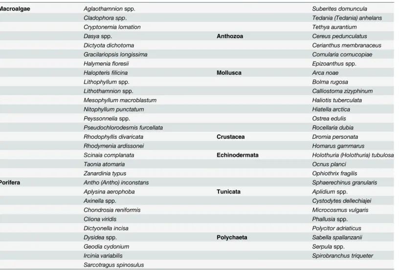
The most frequent and widespread taxa found on the northern Adriatic calcareous bio-con-cretions are reported inTable 2.
Habitat types. According to expert judgment, 3 dominant epibenthic assemblages have been distinguished (Fig 2).
The first group of reefs (Habitat A) is distinguished by opportunistic and tolerant macroal-gal species that are resistant to mud and organic matter (i.e., turf-forming algae such as Clado-phorasp.,Antithamnionsp., andPseudochlorodesmis furcellata); encrusting Porifera [i.e.,
Antho (Antho) inconstans,Dictyonella incisaandMycale (Mycale) massa]; and bioeroders (i.e.,
Clionaspp. andRocellaria dubia). A second group of reefs (Habitat B) is dominated by massive Porifera (i.e.,Chondrosia reniformis,Tedania anhelans, andIrcinia variabilis); erect Tunicata (Aplidium conicumandAplidium tabarquensis); and non-calcareous encrusting algae ( Peys-sonneliaspp.). The third group of reefs (Habitat C) is located in deep offshore waters and is dominated by non-articulated calcareous macroalgae and, to a lesser extent, by the tunicate
Fuzzy clustering
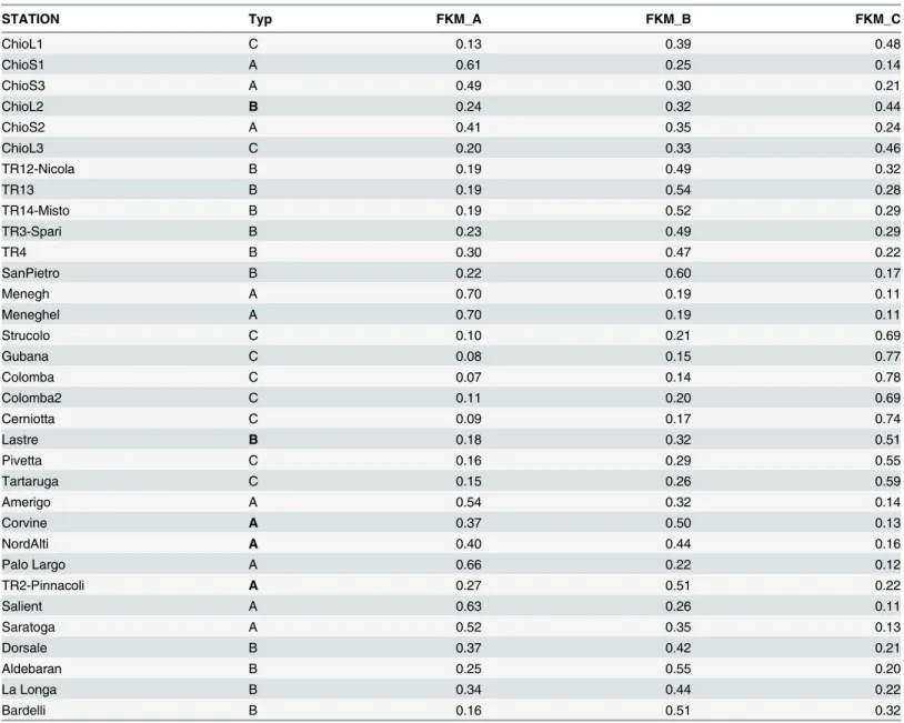
A comparison between the FKM results and the reef types based on expert knowledge is consis-tent (Table 3). Only 5 sites (ChioL2, Lastre, Corvine, Nordalti, and TR2-Pinnacoli) are assigned to a different type by the FKM cluster with the highest fuzzy membership. In all these cases, the expert type assignation is more“conservative”(Fig 2) compared with that of the FKM, i.e., the sites that were assigned by expert knowledge fell in the category immediately below the maxi-mum membership category assigned by the FKM. Furthermore, two of these mismatches occur for sites that the FKM assigned high levels of fuzziness (ChioL2 and Nordalti). Thus, the three FKM clusters have been renamed according to the expert typology. High fuzziness levels, i.e., no membership>0.50, is observed in one-third of the studied sites. Among the remaining
sites, 8 have FKM_A>0.50, 7 have FKM_B>0.50, and 8 have FKM_C>0.50. The FKM_B
clus-ter shows the most restricted membership range (min 0.14–max 0.60); however, both the FKM_A (0.07–0.70) and FKM_C (0.11–0.78) clusters clearly prevail at certain sites, while they show low membership values at other sites. These results supports the interpretation of the FKM_A and FKM_C clusters as the extremes of a gradient that characterizes the epibenthic assemblages on the outcrops. There is also a difference in the mean depth of the reefs of each
Table 2. Common and abundant taxa on northern Adriatic calcareous bio-concretions.
Macroalgae Aglaothamnionspp. Suberites domuncula
Cladophora spp. Tedania (Tedania) anhelans
Cryptonemia lomation Tethya aurantium
Dasyaspp. Anthozoa Cereus pedunculatus
Dictyota dichotoma Cerianthus membranaceus
Gracilariopsis longissima Cornularia cornucopiae
Halymeniafloresii Epizoanthusspp.
Halopterisfilicina Mollusca Arca noae
Lithophyllumspp. Bolma rugosa
Lithothamnionspp. Calliostoma zizyphinum
Mesophyllum macroblastum Haliotis tuberculata
Nitophyllum punctatum Hiatella arctica
Peyssonneliaspp. Ostrea edulis
Pseudochlorodesmis furcellata Rocellaria dubia
Rhodophyllis divaricata Crustacea Dromia personata
Rhodymenia ardissonei Homarus gammarus
Scinaia complanata Echinodermata Holothuria (Holothuria) tubulosa
Taonia atomaria Ocnus planci
Zanardinia typus Ophiothrix fragilis
Porifera Antho (Antho) inconstans Sphaerechinus granularis
Aplysina aerophoba Tunicata Aplidiumspp.
Axinellaspp. Cystodytes dellechiajei
Chondrosia reniformis Microcosmus vulgaris
Cliona viridis Phallusiaspp.
Dictyonella incisa Polycitor adriaticus
Dysideaspp. Polychaeta Sabella spallanzanii
Geodia cydonium Serpulaspp.
Ircinia variabilis Spirobranchus triqueter
Sarcotragus spinosulus
cluster; the FKM_A and FKM_B clusters are found in shallower waters (17.6 m and 18.0 m, respectively), whereas the FKM_C reefs are found in deeper areas (22.6 m).
Direct gradient analysis according to the RDA
The surface chemical-physical model constructed with 14 variables (the median and value ranges for the surface TEMP, SAL, DOX, NTRA, AMON, PHOS, DOX, and CPHL) had an adjusted R2[68,86] of 0.78 (0.63 on the first axis, 0.15 on the second axis, both p<0.001, 999
permutations). Many of the variables were not statistically significant because they presented high collinearity. The forward selection only retained four variables (PHOS, SAL, CPHL, and value range for CPHL) and had an adjusted R2= 0.67 and first axis R2= 0.60 (both axes p<0.01, 999 permutations) (S1 Fig).
The bottom chemical-physical RDA of 14 variables (the median and value ranges for the
bottom TEMP, SAL, DOX, NTRA, AMON, PHOS, DOX, and CPHL) had an adjusted R2of
0.58. The majority of the variance was explained by the first axis (0.49), although both axes were significant (p<0.001, 999 permutations). The forward selection only retained two
vari-ables (value ranges for TEMP and PHOS). The reduced model explained 0.58 of the variance on the first axis and 0.05 of the variance on the second axis (both axes p<0.05, 999
permuta-tions) (S2 Fig).
The hydrodynamic model was built with all 4 hydrodynamic variables (Vmean and Vmax of the surface and bottom). The adjusted R2was 0.23 on the only significant axis (p<0.001, 999
permutations). The forward selection retained only the two surface velocities, and the adjusted R2was 0.26 on the only significant axis (p<0.001, 999 permutations) (S3 Fig).
The final RDA was built using the selected variables of the three RDA subsets: the median surface PHOS, SAL, and CPHL; value ranges for the surface CPHL; and value ranges for the
Fig 2. Dominant epibenthic assemblages of calcareous bio-concretions (Habitat A, Habitat B, and Habitat C) (original copyright 2015).
bottom TEMP and PHOS, surface Vmean and Vmax, and depth. The entire model had an adjusted R2of 0.79; 0.64 of the variance was explained by the first axis, and 0.14 of the variance was explained by the second axis, with both of these values highly significant (p<0.001, 999
permutations). This result was obtained using only 9 variables out of the initial 33. A further forward selection retained only 3 variables (range of phosphate at bottom, mean surface veloc-ity, and surface phosphate), with an adjusted R2of 0.74 on the two significant axes (p<0.001,
999 permutations). In the following, we discuss the final model with 9 partially redundant variables because many of them are of great ecological importance and might be available for comparison in other study areas. For the FKM_A cluster, 0.66 and 0.13 of the variance was explained by the first and second axis, respectively, whereas for the FKM_B cluster, a greater amount of variance was explained by the second axis (0.55) relative to the first axis (0.15). For the FKM_C cluster, almost all of the variance was explained by the first axis (0.93). The high
Table 3. Results of the FKM membership grades (FKM_A, FKM_B, and FKM_C) and habitat typology (Typ) to which the outcrop has been assigned based on expert knowledge (Habitats A, B, and C). The mismatches between the expert typology and the FKM results are in bold.
STATION Typ FKM_A FKM_B FKM_C
ChioL1 C 0.13 0.39 0.48
ChioS1 A 0.61 0.25 0.14
ChioS3 A 0.49 0.30 0.21
ChioL2 B 0.24 0.32 0.44
ChioS2 A 0.41 0.35 0.24
ChioL3 C 0.20 0.33 0.46
TR12-Nicola B 0.19 0.49 0.32
TR13 B 0.19 0.54 0.28
TR14-Misto B 0.19 0.52 0.29
TR3-Spari B 0.23 0.49 0.29
TR4 B 0.30 0.47 0.22
SanPietro B 0.22 0.60 0.17
Menegh A 0.70 0.19 0.11
Meneghel A 0.70 0.19 0.11
Strucolo C 0.10 0.21 0.69
Gubana C 0.08 0.15 0.77
Colomba C 0.07 0.14 0.78
Colomba2 C 0.11 0.20 0.69
Cerniotta C 0.09 0.17 0.74
Lastre B 0.18 0.32 0.51
Pivetta C 0.16 0.29 0.55
Tartaruga C 0.15 0.26 0.59
Amerigo A 0.54 0.32 0.14
Corvine A 0.37 0.50 0.13
NordAlti A 0.40 0.44 0.16
Palo Largo A 0.66 0.22 0.12
TR2-Pinnacoli A 0.27 0.51 0.22
Salient A 0.63 0.26 0.11
Saratoga A 0.52 0.35 0.13
Dorsale B 0.37 0.42 0.21
Aldebaran B 0.25 0.55 0.20
La Longa B 0.34 0.44 0.22
Bardelli B 0.16 0.51 0.32
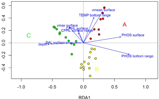
FKM_A and high FKM_C values were observed on opposite ends of the main gradient (Fig 3). This gradient was primarily from high median surface PHOS and high bottom PHOS range values, which are associated with high FKM_A values, toward high depth and high surface salinity values, which are associated with high FKM_C values. The FKM_C sites were posi-tioned offshore at a distance from the effects of river inputs, whereas the FKM_A sites were those closest to the coastline and river inputs. The FKM_B sites were somewhat in the middle of this gradient, but only a rather small fraction of their variance was explained by this gradient. The high range of PHOS may have been related to more shallow areas, where occasional inputs of high river flow can affect the entire water column. Moreover, the bottom sediments in the shallow areas may be easily resuspended by vertical mixing and turbulence caused by waves and wind. The high concentrations of PHOS at depth, which is a signature of remineralization, have previously been described for the northern Adriatic Sea [58,87].
The second axis gradient mainly included the surface Vmean and Vmax, the median surface CPHL, the surface CPHL range, and the bottom TEMP range, with high FKM_B membership grades associated with low values of these variables and FKM_A membership grades associated with high values of these variables. The sites with high FKM_B memberships presented more of an offshore distribution relative to the FKM_A sites; thus, they were less influenced by river-ine waters, which cause strong fluctuations in primary production because of seasonal fluctua-tions in river flow.
A portion of the variance could not be explained by our model, especially for the FKM_B membership grades (S1 Table). The distribution of high FKM_B values (Fig 1) revealed that several sites showing high FKM_A and FKM_B are located close to each other and many are also in the same cell within the 2.5 x 2.5 km grid on which the model was applied. Our resolu-tion was constrained by the scarcity of available data; thus, it could not explain the observed
Fig 3. Final RDA model.Entire model adjusted to R2= 0.79, first axis adjusted R2= 0.64, second axis adjusted R2= 0.14. Both axes are significant at
p<0.001 after 999 permutations(original copyright 2015).
differences between these sites. Moreover, the sites that were poorly fit by our model were found at a distance from each other in different parts of the study domain. This result suggests that certain local factors (e.g., fishing, sedimentation regimes, and endogenous factors such as autocorrelations caused by the clumping/dispersion of organisms) might have contributed to the observed variance in the outcrops.
Our results show that the surface and bottom dynamics are not always decoupled because of the limited depth of the water column in the study area. Thus, appropriate surface or bottom environmental descriptors can provide nearly equivalent explanations of the observed gradi-ents in the outcrops (Table 4) notwithstanding possible causal relationships, which are not accounted for by the RDA. The depth range of the study sites was between 12.4 and 26 m, and even the deepest layers of the water column can be influenced by surface dynamics. Moreover, the height of the outcrops ranged from 0.5 to 4.5 m, and biotic data were collected on horizon-tal surfaces on top of the outcrops, which further reduced the possible effects of depth on the assemblages. In the study area, surface heat loss and wind-driven mixing in autumn and winter tend to homogenize the water column, but intense pulses of freshwater from rivers can induce relevant vertical stratification due to a layer of less saline water at surface. In spring and early summer, the vertical profile of temperature and salinity is strongly stratified with a noticeable
Table 4. Portions of the variance explained by the three groups of variables (surface parsimonious model, bottom parsimonious model, and hydrodynamic parsimonious model) and depth. Only the effects of single groups, combinations of groups, and single groups conditioned to single groups and combinations of groups are shown. The (+) sign indicates that the variance is explained by that combination of variables. The (|) sign indicates that the variance explained by the group on the left is conditional on the variance explained by the group(s) on the right of the sign.
GROUP OF VARIABLES adjusted R2 GROUP OF VARIABLES adjusted R2
Single groups Conditional on 1 group
Surface 0.67 Surface|Bottom 0.09
Bottom 0.63 Surface|Hydro 0.48
Hydro 0.29 Surface|Depth 0.38
Depth 0.33 Bottom|Surface 0.05
Combinations of 2 groups Bottom|Hydro 0.39
Surface+Bottom 0.72 Bottom|Depth 0.30
Surface+Hydro 0.78 Hydro|Surface 0.11
Surface+Depth 0.71 Hydro|Bottom 0.06
Bottom+Hydro 0.68 Hydro|Depth 0.21
Bottom+Depth 0.63 Depth|Surface 0.04
Hydro+Depth 0.54 Depth|Bottom 0.00
Combinations of 3 groups Depth|Hydro 0.25
Surface+Bottom+Hydro 0.79 Conditional on 2 groups
Surface+Bottom+Depth 0.73 Surface|Hydro+Depth 0.23
Surface+Hydro+Depth 0.77 Surface|Bottom+Depth 0.10
Bottom+Hydro+Depth 0.70 Surface|Bottom+Hydro 0.11
All groups of variables Bottom|Hydro+Depth 0.16
All 0.79 Bottom|Surface+Depth 0.03
Residuals (not explained) Bottom|Surface+Hydro 0.02
Residuals 0.21 Hydro|Surface+Depth 0.06
Conditional on 3 groups Hydro|Bottom+Depth 0.07
Surface|Bottom+Hydro+Depth 0.09 Hydro|Surface+Bottom 0.08
Bottom|Surface+Hydro+Depth 0.02 Depth|Bottom+Hydro 0.01
Hydro|Surface+Bottom+Depth 0.05 Depth|Surface+Hydro -0.01
Depth|Surface+Bottom+Hydro 0.00 Depth|Surface+Bottom 0.02
thermocline; however, after strong wind events, the stratification can be broken and the mixed layer can reach the deepest parts of the water column. These wind events are less frequent in spring/summer than in autumn/winter.
The high correlation of depth with selected surface and bottom environmental descriptors
(Table 4) reveals that coastal-related processes, such as river inflows, play an important role in
structuring the assemblages of the outcrops, whereas other processes, such as coastal pollution and recreational and commercial fishing, might also have an important role. In particular, the outcrops are threatened by mechanical damage related to trawling, heavy bottom gear distur-bances, and anchoring. These practices are particularly destructive because of their direct effects, and they also increase the turbidity and sedimentation rates, which negatively affect the structure and composition of the assemblages. Encrusting calcareous macroalgae andPolycitor adriaticus, which are species that characterize Habitat C, are negatively correlated with the mud content of sediment [22,88]. In particular,P.adriaticusis found in undisturbed environments, and its popu-lations are reduced or disappear at increased stress rates. Other tunicates, such asAplidium coni-cum, which characterize Habitat B, are adversely affected by excessive sediment deposition, which causes burial and clogging of the siphons and the branchial wall [88]. Finally, the additive action of silting and high hydrodynamism has injurious consequences because the suspended inorganic particles have a mechanically abrasive effect on living organisms [89]. However, turfs are dominant in areas with increased sedimentation rates [23,79,90]. The abundance of encrust-ing sponges (i.e.,Dictyonella incisa), which, together with turf algae, characterize Habitat A, increased with the mud and organic matter content of nearby sediment, whereas it decreased with increasing distance from the coast and increasing longitude and salinity [22].
Hydrodynamism appears to play an important role that is not shared among any of the other groups of variables (Table 4), and this result might be related to water renewal, advection in nutri-ent rich waters, variations in organism dispersal, and physical constraints on species that can cling onto the substrate. The sites with high FKM_A memberships are found close to the coast; thus, they are strongly affected by coastal currents that flow westward and south-westward in the study area and are seasonally enhanced by surface river inputs and meteorological conditions (easterly winds). These shallower areas display more energetic hydrodynamics throughout the year, whereas the areas characterized by high FKM_C membership appear to be occasionally affected by strong surface velocities that most likely do not affect the bottom assemblages because of the greater bot-tom depth. The FKM_B sites appear to be related to areas of weaker hydrodynamism; however, an inspection of the hydrodynamic subset RDA (S3 Fig) revealed that the FKM_B variance explained by the hydrodynamic variables was negligible. Thus, we can conclude that hydrodynamic variables do not play a role in differentiating FKM_B sites from the other two site clusters.
The onshore-offshore gradient is the most important gradient for explaining the variability of the assemblages growing over northern Adriatic biogenic outcrops because of the extent of coastal freshwater influence, which is the main driver of nutrient dynamics in the Northern Adriatic Sea, and the deepening of the water column in offshore sites, which lessens the sensi-tivity of the bottom population to certain surface dynamics (waves, surface) and is a proxy for the available light provided to the organisms growing on the outcrops. A less important gradi-ent that is more difficult to explain according to the variables used in this study is confined to a coastal belt and differentiates two habitat types, FKM_B and FKM_A, with FKM_A experienc-ing greater exposure to environmental variability.
Predictive model
each fuzzy membership grade were generally consistent among the areas where they were observed (Figs4,5and6).
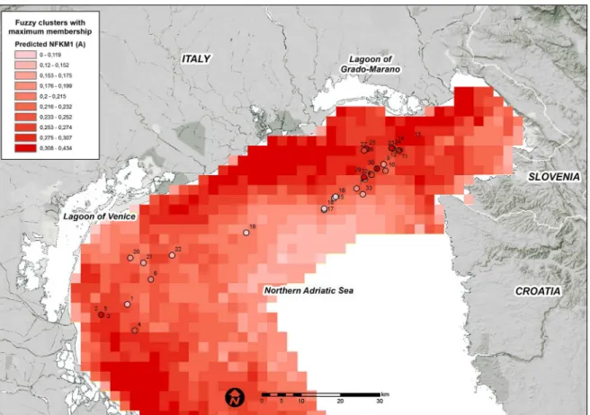
High FKM_A memberships are predicted along the coast, particularly in the north-western and south-western study area (Fig 4). The coastal belt in front of the Venice Lagoon and the Grado-Marano Lagoon are predicted to be less suitable for habitats in FKM_A. A few cells with high predicted FKM_A values are positioned in the Gulf of Trieste close to the mouth of the Isonzo River. In general, high FKM_A memberships appear to favor areas close to freshwater sources and areas at shallow bottom depths.
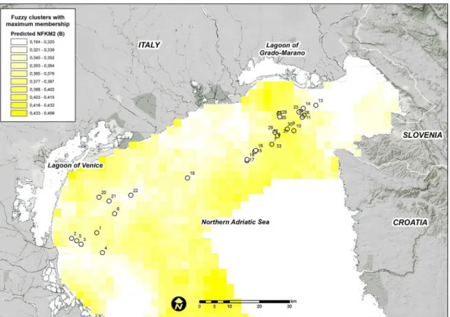
High FKM_C values are predicted offshore, at far distances from rivers and in deeper areas
(Fig 5). In addition, the majority of the Gulf of Trieste as well as the coastal belt in front of the
Venice Lagoon appear to be suitable for this cluster. The higher suitability of FKM_C com-pared with FKM_A in front of the Venice Lagoon might be a result of the buffer effect of the lagoon, which acts as a filter for high-nutrient loads transported to the lagoon from freshwater and from industrial and residential wastes [91,92].
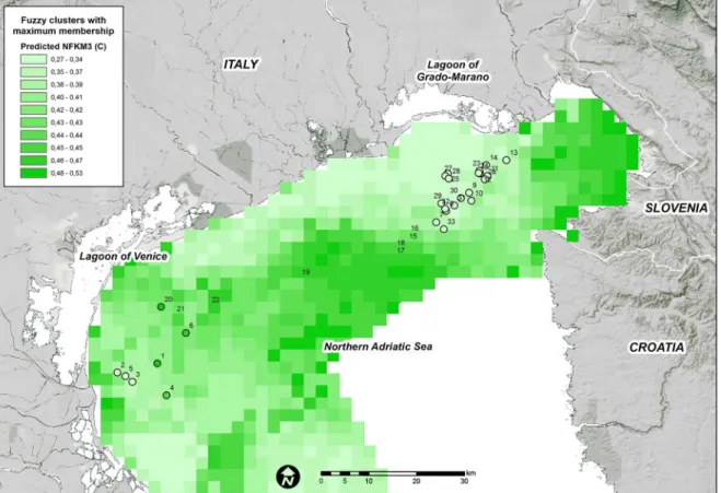
FKM_B is predicted to occur close to the areas where this cluster has been observed, particu-larly in front of the Grado-Marano Lagoon (Fig 1). Nevertheless, the“intermediate” character-istics of the macrobenthic populations on the reefs of this cluster and its lower fit in the final RDA model compared with that of the other two clusters increase its likelihood in areas of the study domain where FKM_A or FKM_C (or both) are not predicted at high values (Fig 6). Areas of transition are a natural feature of the marine environment and may include a mixture of habitats and species.
Fig 4. Predicted FKM_A memberships over the entire study area.Points show the sampling sites used in the present study. White = low membership and dark red = high membership.
The proposed model, that applies to the Italian side of the Northern Adriatic, and the actual occurrence of Habitat A, B, or C in the areas predicted by the model should be assessed with new samplings. Nevertheless, a major constraint that was not included in the model is the pres-ence of a hard substrate. The prespres-ence or abspres-ence of a hard substrate is critical for the develop-ment of epibenthic communities; however, a complete cartography of substrate types in the study area is not available. Thus, our results might be helpful for defining areas worthy of exploration in further research projects.
Because mapping and comparing habitats across geographic regions is a key component of the classification process [15,17], the habitats derived from this study may be suitable for appli-cation in studies focused on other geographic areas. The Apulia continental shelf coralligenous outcrops fall into the“bank”category, which is similar to those in the northern Adriatic, and both contain the same features: isolated blocks randomly scattered on the soft bottom and clus-ters of blocks or ridges with several meclus-ters of lateral continuity [7,23]. These features could rep-resent distinct phases of morphological development [7]. Outcrops with columnar shapes resembling small patch reefs also characterize the bottom off southeast Sicily [6]. If we consider the biotic component, the Apulian outcrops are colonized by coralline algae associated with organisms that also characterize the proposed habitats of the northern Adriatic; however, some of these outcrops show an additional“erect ramified”animal layer, thus representing a fourth complex habitat. The absence of larger bryozoans and gorgonians in the studied area is most likely related to the increased sediment resuspension, the reduced surface of colonization, and the high water turbidity.
Fig 5. Predicted FKM_C memberships over the entire study area.Points show the sampling sites used in the present study. White = low membership and dark green = high membership.
Information on marine habitats must play a major role in ecosystem-based management promoted at national and international levels [93,94]. The three habitats proposed here are easy to identify in the field, and we have related these habitats to different environmental fea-tures (i.e., geography, nutrients, salinity, and temperature). We have also developed a predic-tive model based on environmental features, thus providing a large-scale probabilistic model of the presence of these different habitats in the northern Adriatic basin.
Supporting Information
S1 Checklist. Macroalgae reference checklist. (XLS)
S2 Checklist. Epibenthic fauna reference checklist. (XLS)
S1 Fig. Surface chemical-physical parsimonious RDA model.The adjusted R2value for the entire model is 0.67, with 0.60 on the first axis and 0.07 on the second axis. Both axes are signif-icant (p<0.01, 999 permutations).
(TIFF)
S2 Fig. Bottom chemical-physical parsimonious RDA model.The adjusted R2value for the entire model is 0.63, with 0.58 on the first axis and 0.03 on the second axis. Both axes are
Fig 6. Predicted FKM_B memberships over the entire study area.Points show the sampling sites used in the present study. White = low membership and dark blue = high membership.
significant (p<0.05, 999 permutations).
(TIFF)
S3 Fig. Hydrodynamic parsimonious RDA model.The first (and only significant) axis (p<0.001, 999 permutations) has an adjusted R2= 0.26.
(TIFF)
S1 Table. Fraction of the variance explained in the sampling sites.FKM is the fuzzy cluster with the highest membership at each site. RDA1 and RDA2 are the fractions of the variance explained by each axis, and TOT is the total fraction of the variance explained by the entire model.
(DOC)
Author Contributions
Conceived and designed the experiments: AF SK VB CS. Performed the experiments: AF SK GG SQ VB. Analyzed the data: AF SK DC CM SM GG SQ VB. Contributed reagents/materials/ analysis tools: SQ VB CS. Wrote the paper: AF SK EB VB.
References
1. Ballesteros E. Mediterranean coralligenous assemblages: a synthesis of present knowledge. Oceanogr Mar Biol Annu Rev. 2006; 44: 23–195.
2. Bosence DWJ. Coralline algal reef frameworks. J Geol Soc Lond. 1983; 140: 365–376.
3. Bosence DWJ. The“coralligène”of the Mediterranean—a recent analogue for tertiary coralline algal
limestones. In: Toomey DF, Nicketi MH, editors. Paleoalgology: contemporary research and applica-tions. Heidelberg: Springer-Verlag; 1985. pp. 216–225.
4. Di Geronimo I, Di Geronimo R, Rosso A, Sanfilippo R. Structural and taphonomic analysis of a colum-nar coralline algal build-up from SE Sicily. Geobios Mem Spec. 2001; 35: 86–95.
5. Di Geronimo I, Di Geronimo R, Improta S, Rosso A, Sanfilippo R. Preliminary observation on a colum-nar coralline build-up from off SE Sicily. Biologia Marina Mediterranea. 2001; 8: 229–237.
6. Di Geronimo I, Di Geronimo R, Rosso A, Sanfilippo R. Structural and taphonomic analyses of a colum-nar coralline algal build-up from SE Sicily. Geobios. 2002; 24: 86–95.
7. Bracchi V, Savini A, Marchese F, Palamara S, Basso D, Corselli C. Coralligenous habitat in the Medi-terranean Sea: a geomorphological description from remote data. Ital J Geosci. 2015; 134.
8. Pérès J, Picard JM. Nouveau manuel de bionomie benthique de la mer Méditerranée. Recueil des
Tra-vaux de la Station Marine d’Endoume 1964; 31: 1–131.
9. Laborel J. Marine biogenic constructions in the Mediterranean. Scientific Reports of Port-Cros National Park 1987; 13: 97–126.
10. UNEP-MAP-RAC/SPA. Action plan for the conservation of the coralligenous and other calcareous bio-concretions in the Mediterranean Sea. Tunis: RAC/SPA; 2008.
11. Kipson S, Fourt M, Teixidó N, Cebrian E, Casas E, Ballesteros M, et al. Rapid biodiversity assessment and monitoring method for highly diverse benthic communities: a case study of Mediterranean coralli-genous outcrops. PLoS One. 2011; 6: e27103. doi:10.1371/journal.pone.0027103PMID:22073264 12. Salomidi M, Katsanevakis S, Borja A, Braeckman D, Damalas D, Galparsoro I, et al. Assessment of
goods and services, vulnerability, and conservation status of European seabed biotopes: a stepping stone towards ecosystem-based marine spatial management. Mediterr Mar Sci. 2012; 13: 49–88.
13. Canals M, Ballesteros E. Production of carbonate sediments by phytobenthic communities in the Mallorca-Minorca Shelf, northwestern Mediterranean Sea. Deep Sea Res Part II. 1997; 44: 611–629. 14. Martin CS, Giannoulaki M, De Leo F, Scardi M, Salomidi M, Knitweiss L, et al. Coralligenous and maerl
habitats: predictive modelling to identify their spatial distributions across the Mediterranean Sea. Sci Rep. 2014; 4: 5073.
15. Costello MJ. To know, research, manage, and conserve marine biodiversity. Oceanis. 2001; 24: 25–
49.
17. Costello MJ, Emblow C. A classification of inshore marine biotopes. In: Wilson JG, editor. The intertidal ecosystem: the value of Ireland’s shores. Dublin: Royal Irish Academy; 2005. p 25–35.
18. Moss D, Wyatt BK. The CORINE biotopes project: a database for conservation of nature and wildlife in the European community. Appl Geogr. 1994; 14: 327–349.
19. Borg JA, Schembri PJ. Alignment of marine habitat data of the Maltese Islands to conform to the requirements of the EU habitats directive (Council Directive 92/43/EEC). [Report Commissioned by the Malta Environment and Planning Authority]. Malta: Independent Consultants; 2002. 136pp + Figs 1-23SaràM. 1969. Il coralligeno pugliese e I suoi rapporti con l’ittiofauna. Bollett. Mus. Istit. Biol. Univ.
Genova 37: 27–33
20. Davies CE, Moss D. EUNIS habitat classification. Final report to the European Topic Center on Nature Conservation. Copenhagen: European Environment Agency; 1999.
21. Casellato S, Stefanon A. Coralligenous habitat in the northern Adriatic Sea: an overview. Mar Ecol. 2008; 29: 321–341.
22. Ponti M, Fava F, Abbiati M. Spatial-temporal variability of epibenthic assemblages on subtidal biogenic reefs in the northern Adriatic Sea. Mar Biol. 2011; 158: 1447–1459.
23. Curiel D, Falace A, Bandelj V, Kaleb S, Solidoro C, Ballesteros E. Spatial variability of macroalgal coral-ligenous assemblages on biogenic reefs in the northern Adriatic Sea Bot Mar. 2012; 55: 625–638.
24. Elith J, Phillips SJ, Hastie T, Dudık M, Chee Y, Yates CJ. A statistical explanation of MaxEnt for
ecolo-gists. Divers Distrib. 2011; 17: 43–57.
25. Guisan A, Zimmermann NE. Predictive habitat distribution models in ecology. Ecol Model. 2000; 135: 147–186.
26. Franklin J, Miller J. Statistical methods—modern regression. In: Franklin J, editor. Spatial inference and
prediction with biogeographical data. Cambridge: Cambridge University Press; 2009. p. 113–153. 27. Davies AJ, Guinotte JM. Global habitat suitability for framework-forming cold-water corals. PLoS ONE.
2011; 6: e18483. doi:10.1371/journal.pone.0018483PMID:21525990
28. Giakoumi S, Sini M, Gerovasileiou V, Mazor T, Beher J, Possingham HP, et al. Ecoregion-based con-servation planning in the Mediterranean: dealing with large-scale heterogeneity. PLoS One. 2013; 8: e76449. doi:10.1371/journal.pone.0076449PMID:24155901
29. Artegiani A, Bregant D, Paschini E, Pinardi N, Raicich F, Russo A. The Adriatic Sea general circulation. Part II: baroclinic circulation structure. J Phys Oceanogr. 1997; 27: 1515–1532.
30. Russo A, Artegiani A. Adriatic Sea hydrography. Sci Mar. 1996; 60: 33–43.
31. Zore-Armanda M. Water exchange between the Adriatic Sea and Eastern Mediterranean. Deep Sea Res. 1969; 16: 171–178.
32. Burba N, Cabrini M, Del Negro P, Fonda Umani S, Dilani L. Variazioni stagionali del rapporto N/P nel Golfo di Trieste. In: Albertelli G, Cataneo-Vietti R, Picazzo M, editors. Atti X Congresso Associazione Italiana Oceanologia Limnologia, Alassio, 1994; p. 333–344.
33. Braga G, Stefanon A. Beachrock e Alto Adriatico: aspetti paleogeografici, climatici, morfologici ed eco-logici del problema. Atti Istit Ven.Sci, Lett Art, Class Sci Mat Nat. 1969; 77: 351–361.
34. Stefanon A. Formazioni rocciose del bacino dell'Alto Adriatico. Atti Istit Ven Sci Lett Arti 1967; 125: 79–
89.
35. Stefanon A. The role of beachrock in the study of the evolution of the North Adriatic Sea. Mem Biogeogr Adriat. 1970; 8: 79–99.
36. Newton R, Stefanon A. The‘Tegnue de Ciosa’area: patch reefs in the Northern Adriatic Sea. Mar Geol. 1975; 8: 27–33.
37. Colantoni P, Gabbianelli G, Ceffa L, Ceccolini C. Bottom features and gas seepages in the Adriatic Sea. In: Proceedings VthInternational Conference on Gas in Marine Sediments, Bologna, 9
–12 Sep-tember, 1998, p. 28–31.
38. Conti A, Stefanon A, Zuppi GM. Gas seeps and rock formation in the northern Adriatic Sea. Cont Shelf Res. 2002; 22: 2333–2344.
39. Gordini E, Marocco R, Tunis G, Ramella R. The cemented deposits of the Trieste Gulf (Northern Adri-atic Sea): areal distribution, geomorphologic characteristics and high resolution seismic survey. J Quat Sci. 2004; 17: 555–563.
40. Gordini E, Falace A, Kaleb S, Donda F, Marocco R, Tunis G. Methane-related carbonate cementation of marine sediments and related macroalgal coralligenous assemblages in the Northern Adriatic Sea. In: Harris PT, Baker EK, editors. Seafloor geomorphology as benthic habitat: geohab atlas of seafloor geomorphic features and benthic habitats. Amsterdam: Elsevier; 2012. p. 185–200.
42. Curiel D, Orel G, Marzocchi M. Prime indagini sui popolamenti algali degli affioramenti rocciosi del Nord Adriatico. Boll Soc Adriat Sci. 2001; 80: 3–16.
43. Curiel D, Molin E. Comunitàfitobentoniche di substrato solido. In: Agenzia Regionale per la
Preven-zione e protePreven-zione Ambientale del Veneto ARPAV (eds.) Le tegnùe dell’Alto Adriatico: valorizzazione della risorsa marina attraverso lo studio di aree di pregio ambientale. Venice: ARPAV; 2010. p. 62–79. 44. Curiel D, Rismondo A, Miotti C, Checchin E, Dri C, Cecconi G, et al. Le macroalghe degli affioramenti
rocciosi (tegnùe) del litorale veneto. Lavori Soc Ven Sc Nat. 2010; 35: 39–55.
45. Curiel D, Checchin E, Dri C, Miotti C, Rismondo A, Mizzan L, et al. Le macroalghe degli affioramenti roc-ciosi (tegnùe) antistanti le bocche di porto della Laguna di Venezia. Boll Mus Civ St. Nat Venezia 2010; 61: 5–20.
46. Ponti M, Mescalchin P. Meraviglie sommerse delle "Tegnùe". Guida alla scoperta degli organismi marini. Associazione "Tegnùe di Chioggia"—onlus. Imola: Editrice La Mandragora; 2008. 47. Solazzi A, Tolomio C. Alghe bentoniche delle“tegnue de Ciosa”. Adriatico Nord-occidentale. Stud
Trent Sci Nat. 1981; 58: 463–470.
48. Gabriele M, Bellot A, Gallotti D, Brunetti R. Sublittoral hard substrate communities of the northern Adri-atic Sea. Cah Biol Mar. 1999; 40: 65–76.
49. Casellato S, Masiero L, Sichirollo E, Soresi S. Hidden secrets of the Northern Adriatic:‘‘Tegnùe”, pecu-liar reefs. Cent Eur J Biol. 2007; 2: 122–136.
50. Casellato S, Sichirollo E, Cristofoli A, Masiero L, Soresi S. Biodiversita`delle‘‘tegnu`e”di Chioggia,
zona di tutela biologica del Nord Adriatico. Biologia Marina Mediterranea. 2005; 12: 69–77. 51. Ponti M, Falace A, Rindi F, Fava F, Kaleb S. Beta diversity pattern in Northern Adriatic Coralligenous
outcrops. In: Proceedings of the Second Mediterranean Symposium on the Conservation of Coralligen-ous and Other CalcareCoralligen-ous Bio-concretions; 2014. p. 147–152.
52. Mizzan L. Malacocenosi e faune associate in due stazioni altoadriatiche a substrati solidi. Boll Mus Civ Stor Nat Ven. 1992; 41: 7–54.
53. Faresi L. Macrozoobenthos. In: Ciriaco S, Gordini E, editors. Trezze o“Grebeni“: biotopi e geotopi dell'Alto Adriatico. Trieste: ArtGroup Trieste; 2010. p. 69–71.
54. ARPAV–Fondazione Musei Civici Venezia. Le tegnùe dell’Alto Adriatico: valorizzazione della risorsa marina attraverso lo studio di aree di pregio ambientale. Venice: Stamperia Cedit S.r.l.; 2010. 55. Magistrato Alle Acque di Venezia–Corila-SELC. Studio B.6.72 B/I. Attivitàdi rilevamento per il
monitor-aggio degli effetti prodotti dalla costruzione delle opere alle bocche lagunari. Rapporto variabilitàattesa.
Area: Ecosistemi di Pregio. Macroattività: Affioramenti rocciosi, Tegnùe. 2006. Available:http://pub.
corila.it/DocumentiPubblici/Monitoraggio/13_MAVeCVN/RapportiValutazione/RapportoVariabilita00/ Tegnue-RapportoVariabilita.pdf
56. Bezdek JC. Pattern recognition with fuzzy objective function algorithms. New York: Plenum Press; 1981.
57. Ferraro MB, Giordani P. A toolbox for fuzzy clustering using the R programming language. Fuzzy Sets and Systems; 2015. In press, doi:10.1016/j.fss.2015.05.001
58. Solidoro C, Bastianini M, Bandelj V, Codermatz R, Cossarini G, Melaku Canu D, Ravagnan E, et al. Current state, scales of variability, and trends of biogeochemical properties in the northern Adriatic Sea. J Geophys Res. 2009; 114: C07S91.
59. Querin S, Cossarini G, Solidoro C. Simulating the formation and fate of dense water in a mid latitude marginal sea during normal and warm winter conditions. J Geophys Res Oceans. 2013; 118: 885–900.
60. QGIS Development Team. QGIS geographic information system. Open Source Geospatial Foundation Project. 2015. Available:http://qgis.osgeo.org.
61. van den Wollenberg AL. Redundancy analysis. An alternative for canonical correlation analysis. Psy-chometrika. 1977; 42: 207–219.
62. Rao CR. The use and interpretation of principal component analysis in applied research. Sankhyaá, Ser A. 1964; 26: 329–358.
63. Bandelj V, Solidoro C, Curiel D, Cossarini G, Melaku Canu D, Rismondo A. Fuzziness and heterogene-ity of benthic metacommunities in a complex transitional system. PLoS One 2012; 7: e52395. doi:10. 1371/journal.pone.0052395PMID:23285023
64. Legendre P, Gallagher ED. Ecologically meaningful transformations for ordination of species data. Oecologia. 2001; 129: 271–280.
65. Legendre P, Legendre L. Numerical ecology, 3rd ed. Developments in environmental modelling. Amsterdam: Elsevier; 2012.
67. Peres-Neto PR, Legendre P, Dray S, Borcard D. Variation partitioning of species data matrices: estima-tion and comparison of fracestima-tions. Ecology. 2006; 87: 2614–2625. PMID:17089669
68. Blanchet FG, Legendre P, Borcard D. Forward selection of explanatory variables. Ecology. 2008; 89: 2623–2632. PMID:18831183
69. Borcard D, Legendre P, Drapeau P. Partialling out the spatial component of ecological variation. Ecol-ogy. 1992; 73: 1045–1055.
70. Oksanen J, Guillaume Blanchet F, Kindt R, Legendre P, Minchin PR, O'Hara RB, et al. vegan: commu-nity ecology package. R package version 2.2–1. 2015. Available:http://CRAN.R-project.org/package=
vegan.
71. Dray S, Dufour AB. The ade4 package: implementing the duality diagram for ecologists. J Stat Soft-ware. 2007; 22: 1–20.
72. Dray S. spacemakeR: Spatial modelling. R package version 0.0-5/r113. 2013. Available: http://R-Forge.R-project.org/projects/sedar/. Accessed:http://www.gebco.net/data_and_products/gridded_ bathymetry_data/gebco_30_second_grid/British Oceanographic Data Center, Liverpool, U.K. 73. Falace A, Kaleb S, Curiel D. Implementazione dei S.I.C. marini italiani. Biologia Marina Mediterranea.
2009; 16: 82–83.
74. Falace A, Curiel D, Sfriso A. Study of the macrophyte assemblages and application of phytobenthic indices to assess the ecological status of the Marano-Grado Lagoon (Italy). Mar Ecol. 2009; 30: 480–
494.
75. Sfriso A, Curiel D. Check-list of marine seaweeds recorded in the last 20 years in the Venice lagoon and comparison with the previous records. Bot Mar. 2007; 50: 22–58.
76. Sfriso F, Curiel D, Rismondo A. The lagoon of Venice. In: Cecere E, Petrocelli A, Izzo G, Sfriso A, edi-tors. Flora and vegetation of the Italian transitional water systems. Spinea: Ed. CORILA, Multigraf; 2009. p. 17–80.
77. Curiel D, Bellemo G, Marzocchi M, Iuri M, Scattolin M. Benthic marine algae of the inlets of the lagoon of Venice (Northern Adriatic Sea—Italy) concerning environmental conditions. Acta Adriat. 1999; 40: 111–121.
78. Curiel D, Miotti C, Marzocchi M. Distribuzione quali-quantitativa delle macroalghe dei moli foranei della Laguna di Venezia. Boll Mus Civ Stor Nat Ven. 2009; 59: 3–18.
79. Falace A, Alongi G, Cormaci M, Furnari G, Curiel D, Ester C, Petrocelli A. Changes in the benthic algae along the Adriatic Sea in the last three decades. Chem Ecol. 2010; 26: 77–90.
80. Boudouresque CF. Recherches de bionomie analytique, structurale et expérimentale sur les peuple-ments benthiques sciaphiles de Méditerranée Occidentale (fraction algale). Les peuplepeuple-ments scia-philes de mode relativement calme sur substrats durs. Bulletin du Muséum d’Histoire Naturelle de
Marseille 1973; 33: 147–225.
81. Ballesteros E. Els vegetals i la zonació litoral: espècies, comunitats i factors que influeixen en la seva
distribució. Arxius Secció Ciències 101, 1–616. Barcelona: Institut d’Estudis Catalans; 1992.
82. Hong JS. Étude faunistique d’un fond de concrétionnement de type coralligène soumisàun gradient
de pollution en Méditerranée nord-occidentale (Golfe de Fos). Doctoral Thesis, Université d’ Aix-Mar-seille II. 1980.
83. Pérès J, Picard JM. Recherches sur les peuplements benthiques de la Méditerranée nord-orientale.
Annales de l’Institut Océanographique de Monaco 1958; 34: 213–291.
84. Orlando-Bonaca M, Lipej L, Malej A, Francé J,Čermelj B, Bajt O, et al. Začetna presoja stanja slovens-kega morja. Poročilo začlen 8 Okvirne direktive o morski strategiji (Initial assessment of Slovenian marine waters. Report for Article 8 of the MSFD). Report 140. Piran, Slovenia: Marine Biology Station, National Institute of Biology; 2012.
85. Bianchi CN. La biocostruzione negli ecosistemi marini e la biologia marina italiana. Biol. Mar. Mediterr. 2001; 8 (1): 112–130.
86. Ezekiel M. Methods of correlation analysis. New York: Wiley; 1930.
87. Solidoro C, Bandelj V, Barbieri P, Cossarini G, Fonda Umani S. Understanding dynamic of biogeo-chemical properties in the northern Adriatic Sea by using self-organizing maps and k-means clustering. J Geophys Res. 2007; 112: C07S90.
88. Naranjo SA, Carballo JL, Garcia-Gomez JC. Effects of environmental stress on ascidian populations in Algeciras Bay (southern Spain). Possible marine bioindicators? Mar Ecol Prog Ser. 1996; 144: 119–
131.
90. Balata D, Piazzi L, Cecchi E, Cinelli F. Variability of Mediterranean coralligenous assemblages subject to local variation in sediment deposition. Mar Environ Res. 2005; 60: 403–421. PMID:15924991
91. Solidoro C, Pastres R, Cossarini G, Ciavatta S. Seasonal and spatial variability of water quality parame-ters in the lagoon of Venice. J Mar Syst. 2004; 51: 7–18.
92. Solidoro C, Bandelj V, Cossarini G, Melaku Canu D, Trevisani S, Bastianini M. Biogeochemical proper-ties in the coastal area of the northwestern Adriatic Sea. In: Campostrini P, editor. Scientific research and safeguarding of Venice 2007 Corila Research Programme 2004–2006 volume VI 2006 results. Venice: Corila; 2007. p. 371–384.
93. Connor DW, Breen J, Champion A, Gilliland PM, Huggett D, Johnston, C, et al. Rationale and criteria for the identification of nationally important marine nature conservation features and areas in the UK. Version 02.11. Peterborough: Joint Nature Conservation Committee (on behalf of the statutory nature conservation agencies and Wildlife and Countryside Link) for the Defra Working Group on the Review of Marine Nature Conservation; 2002.