MAXSTALEY LENINYURI NEVES
A Condition-Based Maintenance
Policy and Input Parameters
Estimation for Deteriorating Systems
under Periodic Inspection
Universidade Federal de Minas Gerais Escola de Engenharia
Programa de P´os-Gradua¸c˜ao em Engenharia El´etrica
A Condition-Based Maintenance
Policy and Input Parameters
Estimation for Deteriorating Systems
under Periodic Inspection
Maxstaley Leninyuri NevesDisserta¸c˜ao de mestrado submetida ao Programa de P´os-Gradua¸c˜ao em Engenharia El´etrica da Universidade Federal de Minas Gerais, como requi-sito parcial `a obten¸c˜ao do T´ıtulo de Mestre em Engenharia El´etrica.
´
Area de Concentra¸c˜ao: Engenharia de Computa¸c˜ao e Telecomunica¸c˜oes Linha de Pesquisa: Sistemas de Com-puta¸c˜ao
Orientador: Prof. Dr. Carlos A. Maia Co-Orientador: Prof. Dr. Leonardo P. Santiago
Acknowledgments
I would like to acknowledge my supervisors, Professors Carlos A. Maia and Leonardo P. Santiago, who each in their way supported me in this work. I am greatly thankful for their guidance and support. I am also thankful to Pro-fessors Benjamim R. Menezes and Marta A. Freitas, dissertation committee members, for the careful review and extremely useful feedback.
This research was partially supported by the Laborat´orio de Apoio `a Decis˜ao e Confiabilidade whose people deserve thanks for many discussions and insights, as well as my colleagues at the Programa de P´os-Gradua¸c˜ao em Engenharia El´etrica and at the Programa de P´os-Gradua¸c˜ao em Engenharia de Produ¸c˜ao.
Agradecimentos
Eu gostaria de agradecer aos meus orientadores, Professores Carlos A. Maia e Leonardo P. Santiago, pelo apoio que me foi oferecido, cada um `a sua maneira. Sou muito grato pela orienta¸c˜ao e suporte. Agrade¸co tamb´em aos Professores Benjamim R. Menezes e Marta A. Freitas, membros da banca, pela cuidadosa revis˜ao do texto e pelos importantes coment´arios.
Esta pesquisa contou parcialmente com o apoio do Laborat´orio de Apoio `a Decis˜ao e Confiabilidade, cujas pessoas merecem meus agradecimentos pelas v´arias discuss˜oes e “insights”, da mesma maneira que meus colegas do Pro-grama de Gradua¸c˜ao em Engenharia El´etrica e do ProPro-grama de P´os-Gradua¸c˜ao em Engenharia de Produ¸c˜ao.
Durante meus anos na Universidade Federal de Minas Gerais eu tive a oportunidade de interagir com v´arias pessoas que influenciaram minha edu-ca¸c˜ao. Eu gostaria de agradecer a todo(a)s, especialmente aos meus ex-orientadores de pesquisa/monitoria e ex-professores.
Abstract
We study the problem of proposing Condition-Based Maintenance policies for machines and equipments. Our approach combines an optimization model and input parameters estimation from empirical data.
The system deterioration is described by discrete states ordered from the state “as good as new” to the state “completely failed”. At each periodic inspection, whose outcome might not be accurate, a decision has to be made between continuing to operate the system or stopping and performing its preventive maintenance. This decision-making problem is discussed and we tackle it by using an optimization model based on the Dynamic Programming and Optimal Control theory.
We then explore the problem of how to estimate the model input param-eters, i.e., how to adequate the model inputs to the empirical data available. The literature has not explored the combination of optimization techniques and model input parameters, through historical data, for problems with im-perfect information such as the one considered in this work. We develop our formulation using the Hidden Markov Model theory.
Resumo
O foco deste trabalho ´e a defini¸c˜ao de pol´ıticas ´otimas de manuten¸c˜ao pre-ventiva em fun¸c˜ao da condi¸c˜ao do equipamento. Propomos uma abordagem que combina um modelo de otimiza¸c˜ao com um modelo de estima¸c˜ao de parˆametros a partir dos dados de campo.
A condi¸c˜ao do sistema ´e descrita por estados discretos ordenados do “t˜ao bom quanto novo” at´e o estado “completamente falhado”. A cada inspe-¸c˜ao, cujo resultado pode ser impreciso, uma decis˜ao ´e tomada: continuar a opera¸c˜ao ou efetuar a manuten¸c˜ao preventiva. Este problema de tomada de decis˜ao ´e analisado e propomos um algoritmo de otimiza¸c˜ao baseado em Programa¸c˜ao Dinamica-Estoc´astica e Controle ´Otimo.
Em seguida, exploramos o problema de como estimar as entradas do mo-delo, ou seja, como adequar os parˆametros de entrada em fun¸c˜ao dos dados dispon´ıveis. At´e o momento, a literatura n˜ao apresentou uma t´ecnica que lida com otimiza¸c˜ao e estima¸c˜ao de parˆametros de entrada (usando dados hist´oricos) para problemas com informa¸c˜ao imperfeita como o considerado neste trabalho. Desenvolvemos nossa abordagem usando os Modelos Ocultos de Markov.
Ilustramos a aplica¸c˜ao dos modelos desenvolvidos com dados de campo fornecidos por uma empresa de minera¸c˜ao. Os resultados mostram a apli-cabilidade da nossa abordagem. Conclu´ımos o texto apresentando poss´ıveis dire¸c˜oes para pesquisa futura na ´area.
Resumo Estendido
Uma pol´ıtica de manuten¸c˜ao baseada na condi¸c˜ao e estima¸c˜ao de parˆametros de entrada para sistemas sujeitos `a deteriora¸c˜ao e a inspe¸c˜oes peri´odicas.
Introdu¸c˜
ao
As atividades ligadas `a manuten¸c˜ao de m´aquinas e equipamentos s˜ao essen-ciais ao bom funcionamento de uma ind´ustria. Dentre essas atividades destacam-se os programas de manuten¸c˜ao preventiva que visam otimizar o uso e a opera¸c˜ao dos equipamentos e m´aquinas (que ser˜ao referidos neste texto como “sistemas”) atrav´es da realiza¸c˜ao de interven¸c˜oes planejadas.
O objetivo destas interven¸c˜oes ´e reparar os sistemas antes que os mesmos falhem1, garantindo, portanto, o funcionamento regular e permanente da
atividade produtiva. Se por um lado a necessidade da manuten¸c˜ao preventiva ´e clara, por outro a programa¸c˜ao de tais interven¸c˜oes n˜ao ´e t˜ao evidente. Uma grande dificuldade reside na elabora¸c˜ao de um planejamento que determine quando realizar a Manuten¸c˜ao Preventiva (PM).
Manuten¸c˜ao Preventiva pode ser classificada em dois tipos: Manuten¸c˜ao Programada (SM) – ou manuten¸c˜ao baseada no tempo – e Manuten¸c˜ao Baseada na Condi¸c˜ao (CBM) – ou manuten¸c˜ao preditiva. No primeiro caso assume-se que o sistema assume apenas dois estados – n˜ao-falhado e falhado – e a manuten¸c˜ao ´e realizada em intervalos de tempos pr´e-estabelecidos, embora n˜ao necessariamente iguais. Um exemplo deste tipo de pol´ıtica
1
de manuten¸c˜ao ´e a Manuten¸c˜ao Preventiva Programada. No segundo caso (CBM), procura-se usar a informa¸c˜ao da condi¸c˜ao do sistema, atrav´es da an´alise de sintomas e/ou de uma estimativa do estado de degrada¸c˜ao, visando determinar o momento adequado de realizar a manuten¸c˜ao. Assim, a CBM considera que o sistema possui m´ultiplos estados de deteriora¸c˜ao, indo do “t˜ao bom quanto novo” at´e o falhado. Mais informa¸c˜oes podem ser obti-das em (Bloom, 2006; Nakagawa, 2005; Wang and Pham, 2006; Pham, 2003; Smith, 1993; Moubray, 1993)
Propomos nesta disserta¸c˜ao um modelo para formular pol´ıticas CBM em sistemas cuja condi¸c˜ao pode ser estimada. Esta estima¸c˜ao pode ser incerta (n˜ao perfeita), j´a que a hip´otese de conhecimento da condi¸c˜ao real do sis-tema quase sempre n˜ao ´e fact´ıvel. Uma pol´ıtica dita a forma com que as a¸c˜oes devem ser escolhidas ao longo do tempo em fun¸c˜ao das informa¸c˜oes co-letadas. Exploramos este problema usando cadeias de Markov e Programa¸c˜ao Dinˆamica-Estoc´astica (SDP).
Al´em do modelo de otimiza¸c˜ao, prop˜oe-se uma t´ecnica para estima¸c˜ao dos parˆametros de entrada (do modelo de CBM). Isto ´e feito usando a teoria dos Modelos de Markov Ocultos (HMM). A combina¸c˜ao da t´ecnica de estima¸c˜ao com o modelo de otimiza¸c˜ao apresenta certa novidade pois, dentro da bibli-ografia consultada, a grande maioria dos modelos de CBM n˜ao discute como calcular seus parˆametros a partir dos dados de campo.
Assim, a principal contribui¸c˜ao deste trabalho situa-se na jun¸c˜ao de um modelo de CBM com um modelo de inferˆencia dos parˆametros de entrada, enfoque que ainda n˜ao foi explorado na literatura. Esta contribui¸c˜ao torna-se clara no exemplo de aplica¸c˜ao fornecido.
Um Modelo de Manuten¸c˜
ao Baseada na
Con-di¸c˜
ao
Assumindo que a condi¸c˜ao do sistema pode ser discretizada em estados, as-sociamos cada estado a um n´ıvel de degrada¸c˜ao. Periodicamente, obt´em-se uma estima¸c˜ao da condi¸c˜ao, sendo que esta estima¸c˜ao pode ser imperfeita
(diferente do verdadeiro estado do sistema). Nossas outras hip´oteses s˜ao: 1. O sistema ´e colocado em servi¸co no tempo 0 no estado “t˜ao bom quanto
novo”;
2. Todos reparos s˜ao perfeitos, ou seja, ap´os o reparo o sistema volta `a condi¸c˜ao “t˜ao bom quanto novo”;
3. O tempo ´e discreto com rela¸c˜ao a um per´ıodo fixo T, ou seja: Tk+1 =
Tk+T, onde k= 1,2, . . .representak-´esimo tempo amostrado.
Repre-sentaremos o instante de tempo Tk pork;
4. No instante k, o sistema ´e inspecionado a fim de medir sua condi¸c˜ao. Isto pode ser feito medindo uma vari´avel do sistema como vibra¸c˜ao ou temperatura. Assume-se que a vari´avel monitorada ´e diretamente relationada com o modo de falha que ´e analisado;
5. No instantek, uma a¸c˜aouk´e tomada: ouuk =C (continuar a opera¸c˜ao
do sistema) ouuk=S(parar e realizar a manuten¸c˜ao). Assim, o espa¸co
de decis˜ao ´e U ={C, S};
6. Falhas n˜ao s˜ao imediatamente detectadas. Ou seja, se o sistema falha em [k−1, k), isto ser´a detectado apenas no instante k.
N´os consideramos dois horizontes:
• Horizonte de curto prazo: desde o in´ıcio da opera¸c˜ao do sistema (k = 0) at´e a parada do sistema (uk =S).
• Horizonte de longo prazo: definido como os horizontes de curto prazo acumulados ao longo do tempo.
Como assume-se reparo perfeito, otimizar no curto prazo garante a otimiza¸c˜ao em longo prazo. Assim, n´os reiniciamos k toda vez que o sistema ´e parado (uk =S). Ap´os o reparo, o sistema volta `a condi¸c˜ao “t˜ao bom quanto novo”,
Considere que o sistema possua v´arios est´agios de deteriora¸c˜ao 1,2, . . . , L, ordenados do estado “t˜ao bom quanto novo” (1) at´e o estado completamente falhado (L). A evolu¸c˜ao ao longo do tempo da condi¸c˜ao do equipamento segue um processo estoc´astico. Se nenhuma a¸c˜ao ´e tomada e sob a hip´otese de que o estado futuro depende apenas do estado presente (i.e., o passado encontra-se “embutido” no presente), esta evolu¸c˜ao caracteriza um processo estoc´astico markoviano.
Seja ent˜ao {Xk}k≥0 uma cadeia de Markov onde Xk denota o estado do
sistema no instante k e {Xk} modela a deteriora¸c˜ao do sistema ao longo
do tempo. Assim, o espa¸co de estado de Xk ´e X = {1,2, . . . , L} o qual
associamos uma distribui¸c˜ao de probabilidade definida como
aij = Pr[Xk+1=j|Xk=i, uk=C] = Pr[X1=j|X0=i, u0=C],
sendo que PLj=iaij = 1, ∀i, j. Vamos expressar essas probabilidades na
forma matricial. Para tal, seja: A≡[aij].
Seja g(·) uma fun¸c˜ao de custo do sistema definida como o custo a ser pago no instante k caso o sistema se encontre no estado xk e caso a a¸c˜ao
tomada for uk. Esta fun¸c˜ao representa o custo operacional do sistema, o
custo esperado em caso de indisponibilidade devido a falhas (lucro cessante), al´em dos custos de manuten¸c˜ao preventiva e corretiva. Logo:
• Para xk ∈1, . . . , L−1 tem-se:
– uk = C (continuar a operar): g(xk, uk) representa o custo
opera-cional, que pode ser escrito em fun¸c˜ao do estado do sistema;
– uk = S (parar e efetuar a manuten¸c˜ao preventiva): g denota o
custo esperado da manuten¸c˜ao preventiva (incluindo o lucro ces-sante), que tamb´em pode ser escrito em fun¸c˜ao do estado do sis-tema;
• Para xk =L (falhado):
– uk = S: g(·) descreve o custo esperado de manuten¸c˜ao corretiva
incluindo o custo de indisponibilidade durante o reparo;
– uk = C: g(·) representa o custo de indisponibilidade no per´ıodo
[k, k+1), geralmente uma decis˜ao n˜ao ´otima pois implica em n˜ao mais operar o sistema.
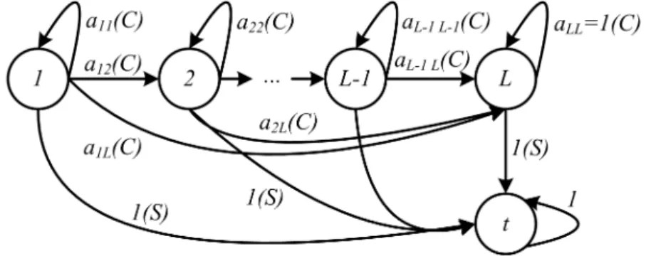
Utilizando os conceitos acima enunciamos a Defini¸c˜ao 1, que descreve as caracter´ısticas de um problema dito bem-definido. Assumiremos que o prob-lema satisfaz esta defini¸c˜ao. A Fig. 3.4 mostra a cadeia de Markov de um problema bem-definido. Pierskalla and Voelker (1976) provaram que sempre existe uma regra de reparo ´otima. Entretanto, para calcul´a-la ´e necess´ario conhecer o estado do sistema Xk a qualquer instante. Como assumimos que
temos apenas uma leitura da condi¸c˜ao do sistema, precisamos utilizar esta informa¸c˜ao para estimar Xk.
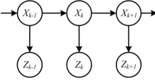
Assim, definimos uma medida de condi¸c˜ao Zk que tem distribui¸c˜ao de
probabilidade condicionada em Xk (veja a Fig. 3.5). Denotamos o espa¸co
de estados de Zk por Z ={1,2, . . . , L}, onde a condi¸c˜ao observada 1
repre-senta “o sistema parece estar no estado 1” e etc.. Seja bx(z) a probabilidade
Pr[Zk = z|Xk = x]. Por conveniˆencia, expressaremos essas probabilidades
na forma matricial: B ≡[bx(z)]. Nota-se queZk representa a liga¸c˜ao entre o
estado do sistema e a(s) vari´avel(is) que monitora(m) o sistema. Conseq¨ uen-temente, uma etapa de classifica¸c˜ao ´e necess´aria convertendo cada valor de medida a um valor de Z. No Cap´ıtulo 5 apresentamos exemplos de classi-fica¸c˜ao.
Definimos um vetor de informa¸c˜aoIk que armazena a condi¸c˜ao estimada
(Zk) desde o in´ıcio da opera¸c˜ao at´e o instante k. Logo, Ik tem tamanho k e
pode ser escrito como
I1 =z1 (1)
Usando este vetor n´os podemos criar um estimador para Xk em qualquer
instante k. Este estimador ´e escrito como
b
Xk = arg max
x∈X Pr[Xk=x|Ik]. (3)
Uma maneira de calcular a probabilidade apresenta acima ´e indicada na Eq. 4.1. Vamos chamar os parˆametros do modelo (A, B) por Ψ. Logo, nesta disserta¸c˜ao, qualquer sistema pode ser integralmente representado pelo seu Ψ e sua fun¸c˜ao de custo g(·).
A pol´ıtica CBM ´otimaµ´e um mapeamento entre a informa¸c˜ao dispon´ıvel e a a¸c˜ao a ser tomada, ou seja,
uk =µ(Ik) =
(
C, if Xbk < r,
S, if Xbk ≥r,
sendo r∈X o estado limite de opera¸c˜ao (ou a regra de reparo). Determinar este limite consiste em resolver o horizonte de curto-prazo. Para tal, pre-cisamos de um algoritmo que minimize o custo acumulado, que ´e resultado da soma dos custos em cada est´agioke influenciado pelas decis˜oes tomadas. Re-solvemos este problema usando Programa¸c˜ao Dinˆamica Estoc´astica (SDP).
Para encontrar a regra de reparo ´otimar, vamos primeiro definirJ como o custo total de opera¸c˜ao do sistema at´e a sua parada, ou seja, a soma de
g(·) at´euk =S. Sob uma dada pol´ıtica µ,J ´e escrito como
Jµ= lim N→∞E
" N X
k=1
αkg(Xk, uk)
#
, (4)
sendo α∈ [0,1] o fator de desconto usado para descontar os custos futuros. O caso mais complexo ´e quando temos α = 1 pois a soma da Eq. 4 pode n˜ao convergir. Entretanto, na Proposi¸c˜ao 2 mostramos que isso n˜ao acontece se o problema for bem definido e, logo, sempre teremos uma solu¸c˜ao. Para
encontrar a pol´ıtica ´otima, decompomos a Eq. 4 na seguinte equa¸c˜ao de SDP
Jk(Ik) = min uk
n
Eg(Xk, uk)|Ik, uk
+ (5)
αEJk+1(Ik, Zk+1)|Ik, uk
o
, k = 1,2, . . . .
Usamos na equa¸c˜ao acima um procedimento chamado de redu¸c˜ao de um problema de informa¸c˜ao imperfeita em um problema de informa¸c˜ao perfeita. Isso ´e poss´ıvel usando o estimador definido na Eq. 3.
Resolvemos a Eq. 5 utilizando um algoritmo de itera¸c˜ao de valor (VI). Bertsekas (2005); Sutton and Barto (1998); Puterman (1994) descrevem com detalhes este procedimento. O Algoritmo 1 apresenta os passos do VI. Como sa´ıda temos a regra de reparo r que, combinado com o estimador Xbk,
repre-senta a pol´ıtica CBM ´otima.
Como descrito anteriormente, como assumimos reparo perfeito (hip´otese 2), resolvendo o horizonte de curto prazo de forma ´otima garante que otimi-zamos tamb´em o horizonte de longo prazo, j´a que o ´ultimo ´e resultado dos horizontes de custo prazo acumulados ao longo do tempo.
A segunda parte desta disserta¸c˜ao se dedica a estimar os parˆametros do modelo de otimiza¸c˜ao, ou seja, Ψ.
Inferˆ
encia dos Parˆ
ametros do Modelo
Busca-se agora adequar os parˆametros de entrada do modelo CBM para sua aplica¸c˜ao em um dado sistema. Assim, estamos interessados em encontrar uma t´ecnica que utiliza os dados dispon´ıveis e nos dˆe a melhor estima¸c˜ao poss´ıvel.
devido, em particular, ao maduro uso dos HMMs em processamento de sinais. Mais informa¸c˜oes a respeito podem ser encontradas em (Rabiner, 1989; Ephraim and Merhav, 2002; Dugad and Desai, 1996; Baum et al., 1970).
Considere O o conjunto de toda informa¸c˜ao dispon´ıvel sobre o sistema.
O pode ser visto como um conjunto deM seq¨uˆencias de observa¸c˜ao, ou seja,
O = {O1, O2, . . . , OM}, onde Om representa uma seq¨uˆencia de leitura da
condi¸c˜ao do sistema e pode ser escrita comoOm ={z1, z2, . . . , zN}, ondeN ´e
o tamanho da seq¨uˆencia ezn ´e a condi¸c˜ao do sistema observada no instante
n.
A estima¸c˜ao dos parˆametros de entrada Ψ = (A, B) ´e um problema no qual, dado a informa¸c˜ao dispon´ıvel O, deseja-se definir Ψ como uma fun¸c˜ao destes dados. Ou seja, desejamos encontrar Ψ que maximiza a Pr[O|Ψ]. Este problema ´e conhecido na literatura de HMM como problema 3. Para re-solvˆe-lo, assume-se que temos uma estimativa inicial (“palpite”) sobre Ψ, que chamaremos de Ψ0. Este problema pode ser resolvido numericamente
apli-cando um conjunto de f´ormulas conhecidas como f´ormulas de Baum-Welch em homenagem a seus autores.
Primeiro, definimos as seguintes vari´aveis:
• forward: αn(x) = Pr[Z1 =z1, Z2 =z2, . . . , Zn =zn, Xn =x|Ψ];
• backward: βn(x) = Pr[Zn+1 = zn+1, Zn+2 = zn+2, . . . , ZN = zN, XN =
x|Ψ].
Seja γn(x) a probabilidade do sistema estar no estado x no instante n
dado a seq¨uˆencia de observa¸c˜oes On, ou seja, γn(x) = Pr[Xn = x|On,Ψ].
Usando a regra de Bayes tem-se
γk(x) = Pr[Xk=x|On,Ψ] =
Pr[Xk =x, On|Ψ]
Pr[On|Ψ]
= αk(x)βk(x) Pr[On|Ψ]
.
Seja agora ξk(i, j) a probabilidade de o sistema estar no estado i no
in-stante k e realizar a transi¸c˜ao para j em k+1, ou seja, ξk(i, j) = Pr[Xk =
i, Xk+1 =j|On,Ψ], o que implica em (usando a regra de Bayes):
ξk(i, j) =
Pr[Xk =i, Xk+1 =j, On|Ψ]
Pr[On|Ψ]
= αk(i)aijbj(Zk+1)βk+1(j) Pr[On|Ψ]
.
Finalmente, sejam ¯aij e ¯bx(z) os estimadores de aij e bx(z)
respectiva-mente. Podemos escrever estes estimadores como:
• ¯aij = KX−1
k=1
ξk(i, j)/ KX−1
k=1
γk(i)
• ¯bx(z) = K
X
k=1 zk=z
γk(x)/ K
X
k=1
γk(x)
Atrav´es da aplica¸c˜ao das f´ormulas de Baum-Welch, Ψ ´e ajustado de forma a aumentar a Pr[O|Ψ] at´e alcan¸car um valor m´aximo. Isto ´e feito da seguinte maneira:
1. Usando o palpite inicial Ψ0, aplicamos as f´ormulas de Baum-Welch
para a primeira seq¨uˆencia de dados O1. Como resultado, obt´em-se as
estima¸c˜oes ¯aij e ¯bx(z), que chamaremos de Ψ1.
2. Voltamos ao passo 1 usando agora como entrada a estima¸c˜ao dos parˆametros atual (Ψ1) e a pr´oxima seq¨uˆencia de dados (O2).
O Algoritmo 2 apresenta a aplica¸c˜ao sucessiva das f´ormulas de Baum-Welch como descrito acima. Ao final, Pr[O|Ψ] ter´a seu valor m´aximo. Este m´aximo representa o m´aximo da fun¸c˜ao de verossimilhan¸ca e pode ser local ou global, sendo que no ´ultimo caso temos a melhor estima¸c˜ao poss´ıvel com os dados dispon´ıveis.
Um Exemplo de Aplica¸c˜
ao
interna que afeta a produtividade do processo. Esta falha pode ocorrer se a corrente el´etrica consumida ultrapassa um valor fixado pelo fabricante. Em caso de ocorrˆencia da falha em estudo, o equipamento pode at´e funcionar em modo degradado mas a degrada¸c˜ao ter´a sido grande e um reparo complexo ser´a necess´ario para rejuvenescer o equipamento.
Vamos definir o estado falhado (L) como o estado onde ser´a necess´ario executar o reparo complexo para colocar o sistema no estado 1 (“t˜ao bom quanto novo”). A falha analisada pode ser vista como oculta pois ela n˜ao implica necessariamente em parada do sistema. Assume-se que outros mo-dos de falha n˜ao s˜ao relevantes para este estudo. A partir da an´alise do equipamento e tendo em vista limita¸c˜oes t´ecnicas, foi definido que a corrente el´etrica ´e o parˆametro monitorado, que ser´a medido todo dia (per´ıodo de amostragem T).
Os dados de campos foram obtidos a partir do hist´orico de funcionamento de 3 equipamentos distintos mas em condi¸c˜oes de opera¸c˜ao similares. Os dados s˜ao compostos por um total de 11 s´eries de leitura de corrente ao longo do tempo, todas se iniciando com o sistema no estado “t˜ao bom quanto novo”. Duas destas s´eries terminam com o sistema sofrendo uma manuten¸c˜ao preventiva (como discutido na Fig. 3.1a) e as demais s´eries terminam com a falha do equipamento.
A fun¸c˜ao de custo g(xk, uk) ´e apresentada na Tab. 5.2. Lembramos que
ela representa o custo a ser pago por estar no estado xk e tomar a decis˜ao
uk, em cada ´epoca de decis˜ao k. A Fig. 5.5 apresenta os dados de campo
e a Tab. 5.1 mostra o passo de classifica¸c˜ao, onde transformamos o valor do parˆametro de controle (θk) em medida de condi¸c˜ao (Zk). O resultado ´e
apresentado na Fig. 5.6.
A discuss˜ao completa do exemplo de aplica¸c˜ao ´e apresentada no Cap. 5. Nele discutimos passo a passo as etapas das t´ecnicas discutidas do trabalho e ilustramos seus pontos chaves.
Conclus˜
ao e Pesquisa Futura
Neste trabalho discutimos a formula¸c˜ao de pol´ıticas de manuten¸c˜ao baseada na condi¸c˜ao (CBM) para sistemas sujeitos `a deteriora¸c˜ao e a inspe¸c˜oes peri-´odicas. O sistema ´e representado por um processo de Markov com estados discretos e levou-se em considera¸c˜ao que a estima¸c˜ao da condi¸c˜ao do sis-tema pode n˜ao ser perfeita. Apresentamos tamb´em uma discuss˜ao sobre a estima¸c˜ao dos parˆametros tanto de um ponto de vista te´orico quanto pr´atico. O resultado principal da disserta¸c˜ao ´e uma t´ecnica que combina um mo-delo de otimiza¸c˜ao e um momo-delo de inferˆencia a partir dos dados hist´oricos do sistema. Este fato foi ilustrado com a aplica¸c˜ao da metodologia proposta em um problema industrial, no qual discutimos passo a passo as etapas apre-sentadas. Os resultados sugerem uma aplica¸c˜ao industrial vi´avel que reflete a realidade encontrada pelos gestores respons´aveis pela tomada de decis˜ao em manuten¸c˜ao.
Um ponto que acreditamos relevante do nosso trabalho ´e que conseguimos realizar a estima¸c˜ao dos parˆametros do modelo de forma consistente. Alguns artigos na literatura j´a tinham apontado uma potencial aplica¸c˜ao dos Mo-delos de Markov Ocultos (HMM) para modelar a evolu¸c˜ao da condi¸c˜ao dos sistemas em manuten¸c˜ao. N´os expandimos esta id´eia propondo um modelo de otimiza¸c˜ao via Programa¸c˜ao Dinˆamica Estoc´astica (SDP) que combina uma etapa de estima¸c˜ao de parˆametros usando os HMMs. Acreditamos que esta combina¸c˜ao ´e interessante e pode motivar mais pesquisas na ´area.
Contents
Acknowledgments ii
Agradecimentos ii
Abstract iv
Resumo v
Resumo Estendido vi
Contents xvii
List of Figures xix
List of Tables xxi
List of Abbreviations xxii
List of Symbols xxiii
1 Introduction 1
1.1 Background . . . 1
1.2 The Problem Addressed . . . 2
1.3 Contributions of this Dissertation . . . 3
1.4 An Overview of the Dissertation . . . 3
Contents
2 Basic Concepts 4
2.1 Reliability and Maintenance . . . 4
2.2 Optimal Maintenance Models . . . 5
2.3 Related Research on Preventive Maintenance Under Risk for Single-unit Systems . . . 9
2.4 Mathematical Tools . . . 12
3 A Model for Condition-Based Maintenance 20 3.1 Introduction and Motivation . . . 20
3.2 Problem Statement . . . 20
3.3 Mathematical Formulation . . . 24
3.4 Model Analytical Properties . . . 32
4 Inference of Model Parameters 35 4.1 Introduction and Motivation . . . 35
4.2 Model Parameters Estimation . . . 36
4.3 Estimation Properties . . . 39
5 An Application Example 44 5.1 Preliminaries . . . 44
5.2 Initial Parameters Estimation . . . 46
5.3 Testing-Scenarios . . . 51
6 Conclusion, Suggestions for Future Research 56
List of Figures
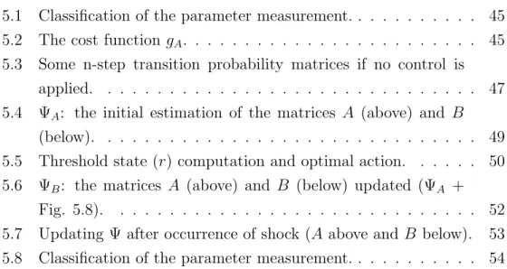
3.1 Condition measurement cycles: up to a preventive mainte-nance (a) and up to a failure (b). . . 21 3.2 The CBM approach proposed in this paper. . . 22 3.3 Long-run horizon optimization. . . 23 3.4 The Markov chain that denotes the system condition
evolu-tion (Xk). The probabilities aij:j>i+1,i<L have been omitted for
succinctness. . . 26 3.5 System state evolution (Xk) and its estimation (Zk). . . 27
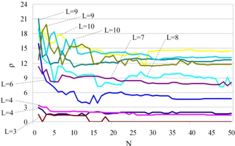
3.6 Stochastic Shortest-Path associated with the problem. . . 30 4.1 Baum-Welch optimal convergence for some random data (10
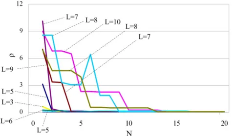
runs). . . 41 4.2 Baum-Welch suboptimal convergence for some random data
(10 runs). . . 42 4.3 Baum-Welch suboptimal convergence for some random data
(1 run). . . 42 4.4 Baum-Welch optimal convergence for some random data (10
runs). . . 43 5.1 The initial guess (Ψ0) of the transition and observation matrices. 46
5.2 The reliability function for the system (Ψ0) if no control is
applied. . . 46 5.3 The failure rate function for the system (Ψ0) if no control is
applied. . . 47
List of Figures
5.4 The distribution of the time to failure (τ(1, L)) for the system (Ψ0) if no control is applied. . . 48
5.5 The data series (total: 11) used in our application example. . . 48 5.6 The same data of Fig. 5.5 after discretization. . . 49 5.7 The reliability (top) and failure rate (middle) functions, and
the distribution of time to failure (bottom) for ΨAif no control
is applied. . . 50 5.8 Scenario 1: condition observed (top) and state estimation
(bottom). . . 51 5.9 Scenario 3: condition observed (top) and state estimation
(bottom). . . 53 5.10 The same data of Figure 5.5 after new discretization (Table
List of Tables
5.1 Classification of the parameter measurement. . . 45 5.2 The cost functiongA. . . 45
5.3 Some n-step transition probability matrices if no control is applied. . . 47 5.4 ΨA: the initial estimation of the matrices A (above) and B
(below). . . 49 5.5 Threshold state (r) computation and optimal action. . . 50 5.6 ΨB: the matrices A (above) and B (below) updated (ΨA +
Fig. 5.8). . . 52 5.7 Updating Ψ after occurrence of shock (A above andB below). 53 5.8 Classification of the parameter measurement. . . 54
List of Abbreviations
CBM: Condition Based Maintenance CM: Corrective Maintenance HHM: Hidden Markov Model LP: Linear Programming MDP: Markov Decision Process PI: Policy Iteration
PM: Preventive Maintenance
RCM: Reliability Centered Maintenance RTF: Run To Failure
SDP: Stochastic Dynamic Programming SM: Scheduled Maintenance
List of Symbols
k The kth time instant . . . 21
L Number of deterioration states . . . 24
Xk System state at epoch k . . . 24
Zk Condition Measured at epoch k . . . 27
uk Action taken at epoch k . . . 21
Ik Information vector at epoch k . . . .27
b
Xk Estimated system state at epoch k . . . 28
A Transition matrix . . . 25
B Condition measurement matrix . . . 27 Ψ System model parameters . . . 28
g Immediate (or step) cost . . . 25
µ Optimal policy . . . 28
r Optimal threshold state . . . 28
J Short-run horizon expected cost . . . .29
O Recorded data compounded by observation sequences . . . 36
Om mth observation sequence . . . 36
Ψ0 Initial guess of the Ψ . . . 38
ΨN Estimation of Ψ after running N observation sequences . . . 38
Chapter 1
Introduction
1.1
Background
Maintenance plays a key role in industry competitiveness. The activities of maintaining military equipments, transportation systems, manufacturing systems, electric power generation plants, etc., often incur high costs and demand high service quality. Consequently, the study of Preventive Main-tenance (PM) has received considerable attention in the literature in the past decades. PM means to maintain an equipment or a machine (here-after denoted as “system”) on a preventive maintenance basis rather than a “let-it-fail-then-fix-it” basis, commonly known as run-to-failure (RTF).
Preventive Maintenance can be classified into two categories: Scheduled Maintenance (SM) (also known as time-based maintenance) and Condition-Based Maintenance (CBM) (or predictive maintenance). The first category considers the system as having two states: non-failed and failed, while the second considers a multi-state deteriorating system. The aim of a SM pol-icy is to derive a statistically fixed “optimal” interval, at which one should intervene in the system (Wang et al., 2008).
Chapter 1: Introduction
of individual systems, which might not follow population-based distributions. Moreover, the SM policy does not include the system condition’s status when the latter is available.
The CBM approach, which is growing in popularity since the 1990s, high-lights the importance of maintenance policies that rely on the conditions (past and present) of systems. In fact, the term CBM denotes monitoring for the purpose of determining the current “health status” of a system’s internal components and predicting its remaining operating life. In other words, on a CBM policy, we try to assess the system’s condition and use this information to propose a more accurate maintenance policy.
1.2
The Problem Addressed
This dissertation proposes a CBM policy and input parameters estimation for deteriorating systems under periodic inspection. Thus, we assume that the system deterioration is described by discrete states ordered from the state “as good as new” to the state “completely failed”. At each periodic inspection, whose outcome might not be accurate, a decision has to be made between continuing to operate the system or stopping and performing its preventive maintenance.
This problem is modeled using the Markov chains theory that, in combi-nation with Stochastic-Dynamic Programming, leads to an optimal solution. An optimal solution is a rule determining when the system should be main-tained, based on its inspection result, in order to minimize its operation cost. We consider that the preventive repair is perfect, that is, it brings back the system to the state “as good as new”. In order to apply our optimiza-tion model, we have formulated an estimaoptimiza-tion technique using the Hidden Markov Models. This estimation allows us to infer about the optimization model parameters using the historical data of the system.
In this context, this dissertation develops a framework combining an op-timization model and input parameters estimation from empirical data.
Chapter 1: Introduction
1.3
Contributions of this Dissertation
The aim of this dissertation is threefold: i) to propose a model to formu-late optimal CBM policies; ii) to develop a procedure for model parameters estimation; and iii) to illustrate our approach with an empirical example.
Our main contribution lies in the fact that we combine an optimization model and a technique for estimating the model input parameters based on system historical data. We believe our approach fills a commonly noticed gap in the literature namely, the fact that most of CBM models do not discuss the model input parameters. Hence, the literature has not explored the combination of optimization techniques and model input parameters, through historical data, for problems with imperfect information such as the one considered in this dissertation.
We argue that our approach is more realistic as far as the estimation of model inputs parameters is concerned. This dissertation also provides a practical discussion using empirical data.
1.4
An Overview of the Dissertation
This dissertation is organized into five chapters. Chapter 2 includes a brief survey of the vast literature in the field of optimal maintenance. This chapter highlights the diversity of approaches proposed to tackle maintenance prob-lems. We also provide in this chapter a brief discussion of the mathematical concepts used in this dissertation.
Chapter 2
Basic Concepts
This chapter provides a briefly description of the maintenance optimization. Different maintenance policies are presented. We also introduce some mathe-matical concepts used in this dissertation.
2.1
Reliability and Maintenance
Reliability engineering studies the application of mathematical tools, spe-cially statistics and probability, for product and process improvement. In this context, researchers and industries are interested in investigating the systems deterioration and how to tackle this phenomenon in order to opti-mize some quantity.
Any system can be classified as repairable and nonrepairable: a nonre-pairable system being a system that fails only once and is then discarded. This work addresses to repairable systems. Since the system can be repaired, it may be wise to plan these repairs, i.e, to plan the maintenance actions.
We are interested in certain quantities for analyzing reliability and main-tenance models. In general, for a given system, we aim to consider three: reliability, availability and maintainability.
Reliability: is defined as the probability that a system will satisfactorily perform its intended function under given circumstances for a speci-fied period of time. Usually, the reliability of a repairable system is measured by its failure intensity function, which is defined as follows
Chapter 2: Basic Concepts
lim
∆t→0
Pr[Number of failures in (t, t+ ∆t]≥1]
∆t .
With this function we can obtain the mean time between failures (MTBF) representing the expected time that the next failure will be observed.
Availability: it means the proportion of time a given system is in a func-tioning condition. The straightforward representation for availability is as a ratio of the expected uptime value to the expected values of the uptime plus downtime, i.e.,
A= E[Uptime]
E[Uptime] + E[Downtime].
Maintainability: is defined as the probability of performing a successful perfect repair within a given time. The mean time to repair (MTTR) is a common measure of the maintainability of a system and it is equals to E[Downtime] under some assumptions.
For additional information on this topic, the reader is referred to (Bloom, 2006; Nakagawa, 2005; Wang and Pham, 2006; Pham, 2003).
2.2
Optimal Maintenance Models
The rise of optimal maintenance studies is closely correlated to the beginning of Operations Research in general which was developed during the Second World War. For example, during this time, a researcher called Weibull fo-cused on approximating probability distributions to model the failure me-chanics of materials and introduced the well-known Weibull distribution for use in modeling component lifetimes.
The literature about optimal maintenance models (continuous or discrete time) can be classified as follows (Sherif and Smith, 1981):
Chapter 2: Basic Concepts
1 Under risk
2 Under uncertainty
a Simple (or single-unit) system
b Complex (or multi-unit) system
i Preventive Maintenance (periodic1, sequential2)
ii Preparedness Maintenance (periodic, sequential, opportunistic3)
Several Applied Mathematics and Computational techniques, such as Op-erations Research, Optimization and Artificial Intelligence, have been em-ployed for analyzing maintenance problems and obtaining optimal mainte-nance policies. We can cite the Linear Programming, Nonlinear Program-ming, Mixed-Integer ProgramProgram-ming, Dynamic ProgramProgram-ming, Search tech-niques and Heuristic approaches.
We define now the concepts of corrective and preventive maintenance. After that we introduce some optimal maintenance models.
2.2.1
Corrective and Preventive Maintenance
Maintenance can be classified into two main categories: corrective and pre-ventive (Wang and Pham, 2006). Corrective Maintenance (CM) is the main-tenance that occurs when the system fails. CM means all actions performed as a result of failure, to restore an item to a specified condition. Some texts refer to CM only as repair. Obviously, CM is performed at unpredictable time points since the system’s failure time is not known.
Preventive maintenance (PM) is the maintenance that occurs when the system is operating. PM means all actions performed in an attempt to retain an item in specified condition by providing systematic inspection, detection, and prevention of incipient failures.
1
In a periodic PM policy, the maintenance is performed at fixed intervals.
2
A sequential PM policy means to maintain the system at different intervals.
3
Opportunistic Maintenance explores the occurrence of an unscheduled failure or repair to maintain the system.
Chapter 2: Basic Concepts
Both CM and PM can be classified according to the degree to which the system’s operating condition is restored by maintenance action in the following way (Wang and Pham, 2006):
1. Perfect repair or perfect maintenance: maintenance actions which re-store a system operating condition to “as good as new”. That is, upon a perfect maintenance, a system has the same lifetime distribution and failure intensity function as a new one.
2. Minimal repair or minimal maintenance: maintenance actions which restore a system to the same level of the failure intensity function as it had when it failed. The system operating state after the minimal repair is often called “as bad as old” in the literature.
3. Imperfect repair or imperfect maintenance: maintenance actions which make a system not “as good as new” but younger. Usually, it is as-sumed that imperfect maintenance restores the system operating state to somewhere between “as good as new” and “as bad as old”.
We briefly present now the characteristics of each optimal maintenance model family.
2.2.2
Deterministic Models
These models are developed under some assumptions, we cite the followings:
• The outcome of every PM is not random and it restores the system to its original state.
• The system’s purchase price and the salvage value are function of the system age.
• Degradation (aging, wear and tear) increases the system operation cost.
Chapter 2: Basic Concepts
The optimal policy for deterministic models is a periodic policy (Sherif and Smith, 1981) and hence the times between PMs are equal. Charng (1981) presents a short discussion on this kind of model, which is is also known as age-dependent deterministic continuous deterioration.
2.2.3
Stochastic Models Under Risk
Risk is a time-dependent property that is measured by probability. For a system subject to failure, it is impossible to predict the exact time of failure. However, it is possible to model the stochastically behavior of the system (e.g. the distribution of the time to failure).
Some of these models will be presented in Section 2.3.
2.2.4
Stochastic Models Under Uncertainty
We deal here with failing systems under uncertainty, i.e., neither the exact time to failure nor the distribution of that time is known. These problems are harder since less information is available. Literature reports methods such as (Sherif and Smith, 1981):
• Minimax techniques: applied when the system is new or failure data are not known;
• Chebychev-type bounds: applied when partial information about the system (such as failure rate) is known;
• Bayesian techniques: applied when subjective beliefs about the system failure and non-quantitative information are available.
Since this dissertation does not deal with this type of problem, this topic will not be covered.
2.2.5
Single-unit and Multi-unit Systems
A simple (single-unit) system is a system which can not be separated into independent parts and has to be considered as a whole. However, in practice,
Chapter 2: Basic Concepts
a system may consist of several components, i.e., the system is compounded by a number of subsystems.
In terms of reliability and maintenance, a complex (multi-unit) system can be assumed to be a single-unit system only if there exists neither eco-nomic dependence, failure dependence nor structural dependence. If there is dependence, then this has to be considered when modeling the system. For example, the failure of one subsystem results in the possible opportunity to undertake maintenance on other subsystems (opportunistic maintenance).
This dissertation considers only single-unit systems or multi-unit systems which can be analyzed as a single-unit one.
2.2.6
Preventive Maintenance Under Risk
In this case we are interested in modeling the system deterioration in order to diagnose the best time to carry out a preventive maintenance. Since this is the focus of this work, we will dedicate the Section 2.3 to cover this theme.
2.2.7
Preparedness Maintenance Under Risk
In preparedness maintenance, a system is placed in storage and it replaces the original system only if a specific but unpredictable event occurs. Some maintenance actions may be taken while the system is in storage and the objective is to choose the sequence of maintenance actions resulting in the highest level of system “preparedness for field use”.
For instance, when the system is in storage, it can be submitted to a long-term cold standby and an objective would be to choose the maintenance actions providing the best level of preparedness (or readiness to use).
2.3
Related Research on Preventive
Mainte-nance Under Risk for Single-unit Systems
Chapter 2: Basic Concepts
a multi-state deteriorating system.
For each category, we discuss the five families of maintenance strategies according to Lam and Yeh (1994):
1. Failure maintenance (Run-To-Failure): no inspection is performed. The system is maintained or replaced only when it is in the failed-state. 2. Age maintenance: the system is subject to maintenance or replacement
at age t (regardless the system state) or when it is in the failed-state, whichever occurs first. The block replacement policy is an example. 3. Sequential inspection: the system is inspected sequentially: the
infor-mation gathered during inspection is used to determine if the system is maintained or the system is scheduled for a new inspection to be performed some time later.
4. Periodic inspection: a special case of sequential, when the period of inspection is constant.
5. Continuous inspection: the system is monitored continuously and when-ever some threshold is reached the system is maintained.
2.3.1
Main Strategies for Two-states Systems
This family of models usually utilizes the following assumptions:
• The time to failure is a random variable with known distribution.
• The system is either operating or failed and failure is an absorbing state: the system only can be regenerated if a maintenance action is performed.
• The intervals between successive regeneration points are independent random variables, i.e., the time between failures are independent.
• The cost of an maintenance action is higher if it is undertaken after failure than before.
Chapter 2: Basic Concepts
Sherif and Smith (1981); Wang and Pham (2006) indicate that failure maintenance is the optimal policy recommended for systems with a constant failure intensity function (exponential). On the other hand, for a system with increasing failure intensity function (weibull or gamma for some parameters) should be maintained or not in function of its age.
The act of using reliability models to plane the maintenance actions is the essence of the Reliability-Centered Maintenance (RCM) (Smith, 1993; Moubray, 1993; Bloom, 2006).
2.3.2
Main Strategies for Multi-states Systems
For multi-state degrading systems, the system is considered to be subject to failure processes which increase the system degradation and random shocks. In this case, we are not only interested in obtaining the system reliability model but also to obtain expressions about the system states by calculating probabilities (Wang and Pham, 2006).
The most common approach is using Markov chains (continuous and dis-crete time) to describe the system. In such approach, the system condition is classified by a finite number of discrete states, such as in Refs. (Kawai et al., 2002; Bloch-Mercier, 2002; Chen et al., 2003; Chen and Trivedi, 2005; Gong and Tang, 1997; G¨urler and Kaya, 2002; Chiang and Yuan, 2001; Ohnishi et al., 1994). The purpose of these models is to determine an action to be carried out at each state of the system (repaired/replaced) in order to obtain a minimum expected maintenance cost.
In terms of the condition measurement, the literature considers sequential checking such as studied in (Bloch-Mercier, 2002; G¨urler and Kaya, 2002), or periodic inspection, such as in (Chen et al., 2003; Gong and Tang, 1997; Chen and Trivedi, 2005; Ohnishi et al., 1994); perfect inspection, such as in (Bloch-Mercier, 2002; Chen and Trivedi, 2005; Chen et al., 2003; Chiang and Yuan, 2001) or imperfect inspection, such as in (Gong and Tang, 1997; Ohnishi et al., 1994).
multi-Chapter 2: Basic Concepts
state systems (Valdez-Flores and Feldman, 1989).
2.4
Mathematical Tools
In this section we briefly introduce some mathematical concepts used in this dissertation. We do not aim to cover these topics comprehensively but just provide a short introduction to them.
2.4.1
Reliability and Statistics
We introduce in this section some statistical terminology for common used in reliability engineering. For the purposes of this section, let T be a non-negative continuous random variable which denotes the first failure time of the system. T has a given probability distributionf(t); the cumulative distri-bution F(t) is called the failure distribution and it describes the probability of failure prior the time t, i.e.,
F(t) = Pr[T ≤t]. (2.1)
The reliability function is defined asR(t) = 1−F(t), which is the proba-bility that the system will continue working past time t. The failure rate (or hazard function) is defined as follows
λ(t) = R(t)−R(t+ ∆t) ∆t·R(t) =
Pr[t < T ≤t+ ∆t|T > t]
∆t , (2.2)
when ∆ →0. It can be shown that λ(t) = Rf((tt)).
This concepts are applied for systems called non-repairable as well as for repairable system when the repair is perfect or the system is simply replaced by a new one. We briefly discuss the two most common models for the failure time. For further information on this topic please check (Rigdon and Basu, 2000; Nakagawa, 2005; Wang and Pham, 2006).
Chapter 2: Basic Concepts
Exponential model
In this model, T is assumed to follow an exponential distribution with a parameter θ. Hence, we have
f(t) = 1
θ exp(−t/θ) and F(t) = 1−exp(−t/θ).
This model has the main features:
1. The memoryless property, i.e., Pr[T ≤ t+a|T ≤ t] = Pr[T ≤ a] = exp(−a/θ);
2. A constant failure rate, i.e,λ(t) = f(t)
R(t) = 1/θ; 3. The expected time to failure (MTTF) is E[T] =θ.
Weibull model
Here we assume that T a weibull distribution with the parameters η and α. Hence,
f(t) = η
α
t α
η−1
exp − t α η
and F(t) = 1−exp
− t α η .
The main properties of this model are:
1. The failure rate isλ(t) = η
α
t α
η−1
;
2. The MTTF is E[T] = αΓ1 + 1
η
, where Γ is the gamma function defined as follows for a a >0:
Γ(a) =
Z ∞
0
Chapter 2: Basic Concepts
2.4.2
Markov Chains
Consider a system that can be in any one of a finite or countably infinite number of states. LetX denote this set of states. Without loss of generality, assume thatX is a subset of the natural numbers ({1, 2, 3, . . .}). X is called the state space of the system. Let the system be observed at the discrete moments of time k = 0,1,2, . . ., and let Xk denote the state of the system
at epoch k.
If the system is non-deterministic we can consider {Xk} (k ≥ 0) as
ran-dom variables defined on a common probability space. The simplest way to manipulate {Xk} is to suppose that Xk are independent random variables,
i.e., future states of the system are independent of past and present states. However, in most system in the practice, this assumption does not hold.
There are systems that have the property that given the present state, the past states have no influence on the future. This property is called the Markov property and one of the most used stochastic processes having this property is called Markov chain. Formally, the Markov property is defined by the requirement that
Pr[Xk+1 =xk+1|X0 =x0, . . . , Xk =xk] = Pr[Xk+1 =xk+1|Xk =xk], (2.3)
for every k ≥ 1 and the states x0, . . . , xk+1 each in X. The conditional
probabilities Pr[Xk+1 =xk+1|Xk =xk] are called the transition probabilities
of the chain.
We call the system’s initial state as ω which is defined by
ω(x) = Pr[X0 =x], x∈X. (2.4)
ωis hence the initial distribution of the chain. If the conditional probabilities depicted in equation 2.3 are constant in time, i.e.,
Pr[Xk+1 =j|Xk =i] = Pr[X1 =j|X0 =i], i, j ∈X, k≥0. (2.5)
Chapter 2: Basic Concepts
the Markov chain is called time-homogeneous. Let us call these probabilities as
aij = Pr[Xk+1 =j|Xk =i], i, j ∈X, k≥0. (2.6)
We define the matrix A ≡ [aij] which is called the transition probabilities
matrix of the (time-homogeneous) chain.
The Markov chains are well-known in the literature mainly because their study is worthwhile from two viewpoints. First, they have a rich theory and, secondly, there are a large number of systems that can be modeled by Markov chains. Further information on this topic can be found in (Hoel et al., 1972; Grimmett and Stirzaker, 2001; Cassandras and Lafortune, 2009).
2.4.3
Hidden Markov Models
In the previous section, we have assumed that we know the system’s state (Xk) any time, i.e., the Markov chain is observable. Indeed, this assumption
has allowed us to state the transition probabilities matrix A (equation 2.6) that, in combination with the initial distribution of the chain, allows us to predict future behavior of the system (e.g. the Chapman-Kolmogorov equation). However, this assumption may not be reasonable for some systems in the practice.
Actually, it is quite common to find a system in which we do not have the directly access to its state. In other words, Xk is unknown or hidden. In this
case, we want to be able to handle this constraint by creating a way to assess
Xk. For this purpose, there have been models which focus on estimatingXk
based on observations.
A Hidden Markov Model (HMM) is a discrete-time finite-state homoge-neous Markov chain ({Xk} in our case) observed through a discrete-time
Chapter 2: Basic Concepts
We denote the set of these observations as Z = {z1, z2, . . . , zL} and we
define the observation probability distribution as
bx(z) = Pr[Zk =z|Xk =x], z∈Z, x ∈X, k ≥0. (2.7)
It is assumed that this distribution does not change over time, i.e., bx(z) is
the same for every k ≥0. These probabilities can be written in a the matrix form: B ≡ bx(z). Hence, a HMM is fully represented by its probability
distributions A, B and ω. For convenience, we define the notation:
Ψ = (A, B, ω). (2.8)
There are three basic problems in HMM that are very useful in practical applications. These problems are:
Problem 1: Given the model Ψ = (A, B, ω) and the observation sequence
O = z1, z2,· · · , zk, how to compute Pr[O|Ψ] (i.e., the probability of
occurrence of O)?
Problem 2: Given the model Ψ = (A, B, ω) and the observation sequence
O =z1, z2,· · · , zk, how to choose a state sequenceI =x1, x2,· · · , xkso
that Pr[O, I|Ψ]4 is maximized (i.e., best “explain” the observations)?
Problem 3: Given the observation sequence O = z1, z2,· · · , zk, how do we
adjust the HMM model parameters Ψ = (A, B, ω) so that Pr[O|Ψ] is maximized?
While problems 1 and 2 are analysis problems, problem 3 can be viewed as a synthesis (or model identification or inference) problem.
The HMMs have various applications and one is pattern recognition such as speech and handwriting. For example, there is a known technique in Signal Processing called the Viterbi Algorithm which efficiently tackles the problem 2. For additional information on this topic, the reader is referred to (Dugad and Desai, 1996; Ephraim and Merhav, 2002; Rabiner, 1989; Grate, 2006).
4
Which represents the joint probability of the state sequence and observation sequence
Chapter 2: Basic Concepts
2.4.4
Applying Control in Markov Chains: Markov
Decision Process
So far, we have considered Markov chains having fixed transition probabili-ties. If we can change these probabilities then we will change the evolution of the chain. In some situations we might be interested in how to induce the system to follow some behavior in order to optimize some quantity. It can be performed if we can “control” the transition probability of the system.
We call the act of controlling the transition probability by applying con-trol in Markov chains. Let us call the concon-trol applied at the timekbyuk ∈U,
U being the control space, i.e, the set of all possible actions. We rewrite Eq. 2.6 taking into account the control as follows
aij(u) = Pr[Xk+1 =j|Xk =i, uk =u], i, j ∈X, u∈U, k ≥0, (2.9)
with Pj∈Xaij(u) = 1, i ∈ X, u∈ U. The control follows a policy denoted
by π, which is nothing but the strategy or a plan of action. In general, a policy is developed using the feedback, i.e., the policy is a plan of actions for each state xk∈X at the time k. Hence, a policy can be written as
π ={µ0, µ1, . . . , µk, . . .}, (2.10)
where µk maps each state to an action, i.e.,µk :xk 7→uk ⇒uk=µk(xk). In
this case, it is assumed that the Markov chain is observable. If µk are all the
same, π is called a stationary policy.
Different policies will lead to different probability distributions. In a optimal control context, we are interested in finding the best or optimal policy. To this end, we need to compare different policies, which can be done by specifying a cost function. Let us assume the cost function is additive. Thus, the total cost until k=n is calculated as follows
n
X
k=0
Chapter 2: Basic Concepts
where g(x, u) is interpreted as the cost to be paid if Xk = x and uk = u
at the time k. g(x, u) is referred to as immediate or one period cost. If the chain (or the system evolution) stops at the time N, there is no action to be taken when k =N and we rewrite Eq. 2.11 as follows
NX−1
k=0
g(xk, uk) +g(xN), (2.12)
g(xN) is called the terminal cost.
Notice thatXk and the actionsukall depend on the choice of the policyπ.
Furthermore, g(xk, uk) is a random variable. If we deal with a finite horizon
problem, for any horizon N, we write the system cost under the policy π as
Jπ(x0) = E
"N−1 X
k=0
g(xk, uk) +gN(xN)
#
, (2.13)
where x0 is the initial state. For an infinite horizon problem, we have
Jπ(x0) = lim
N→∞E
" N X
k=0
g(xk, uk)
#
. (2.14)
Let an optimization problem be the minimization of the expected cost
J. Then, the optimal policy π∗
is that one which minimizes J, i.e., Jπ∗ =
minπJπ. This is a sequential decisions problem that can be tackled using
Dynamic Programming (DP). We will use the term Stochastic Dynamic Pro-gramming (SDP) to reinforce the stochastic character of our problems. SDP decomposes a large problem into subproblems and it is based on the Principle of Optimality proposed by Bellman5. Under this result, the solution of the
general problem is compounded by the solutions of the subproblems.
An explicit algorithm for determining an optimal policy can be developed using SDP. LetJk(xk) be the cumulated cost at timekfor all statesxk. Then,
Jk(xk) = min
uk∈UE [g(xk, uk) +Jk+1(xk+1)], k= 0,1, . . . , (2.15)
5
In Proposition 1, for the purposes of this result, we recall the definition of this principle.
Chapter 2: Basic Concepts
is the optimal cost-to-go from state xk to state xk+1. The function Jk(xk)
is referred to as the cost-to-go function in the following sense: the equation states a single-step problem involving the present costg(xk, uk) and the future
cost Jk+1(xk+1). The optimal action uk is then chosen and the problem is
solved. Of course, Jk+1(xk+1) is not known.
For convenience, let us assume a finite horizon problem. Hence,JN(xN) =
g(xN) is known and it can be used to obtain JN−1(xN−1) by solving the
minimization problem in Eq. 2.15 over uN−1. Then JN−1(xN−1) is used to
obtain JN−2(xN−2) and so on. Ultimately, we obtain J0(x0) which will be
optimal cost. This is a backward procedure.
Some attention is required when working with infinite horizon because the Eq. 2.11 can be infinite or undefined when n→ ∞. Under some circum-stances, the infinite horizon problem does have solution. We illustrate some of such scenarios:
Optimal stopping time (stochastic shortest path): it is assumed that there exist state x and actionu such that g(x, u) = 0.
Expected discounted cost: we use a discounting factor to discount future values. Hence, Eq. 2.14 is replaced by
Jπ(x0) = lim
N→∞E
" N X
k=0
αkg(xk, uk)
#
, α∈(0,1). (2.16)
Expected average cost: a policy is evaluated according to its average cost per unit of time. Hence, Eq. 2.14 is replaced by
Jπ(x0) = lim
N→∞ 1 NE " N X k=0
g(xk, uk)
#
. (2.17)
Chapter 3
A Model for Condition-Based
Maintenance
3.1
Introduction and Motivation
In this chapter we formulate an optimization model for CBM. Our goal is to determine a CBM policy for a given system in order to minimize its long-run operation cost.
3.2
Problem Statement
We assume that the system’s condition can be discretized in states and that each state is associated with a possible degradation degree. Periodically, we have an estimation of the condition, which can be obtained by inspection or by the use of sensor(s) or other devices used to monitor the system. The estimation can be imperfect, that is to say, different from the true system condition. Other assumptions are:
1. The system is put into service in time 0 in the state “as good as new”; 2. All repairs are perfect (for example, by replacing the system), that is, once repaired, the system turns back to the state “as good as new”. We do not consider the minimal-repair possibility;
Chapter 3: A Model for Condition-Based Maintenance
3. The time is discrete (sampled) with respect to a fixed period T, i.e.,
Tk+1 =Tk+T, where k = 1,2, . . . is the kth sample time. In order to
shorten the notation, we denote hereafter the instant time Tk as k ;
4. At the instant k, the system is inspected in order for its condition to be estimated. This inspection may be performed by measuring a system’s variable, e.g., vibration or temperature. The system’s variable monitored is directly related to the failure mode being analyzed; 5. At the instant k, an action uk is taken : either uk = C (continue the
system’s operation, i.e., it is left as it is) or uk=S (stop and perform
the maintenance), i.e., the decision space is U ={C, S};
6. Failures are not instantaneously detected. In other words, if the system fails in [k −1, k), it will be detected only at the epoch k. This is not restrictive since we can overcome this assumption by choosing a small period T.
In our CBM framework, the model parameters are adjusted and the de-cisions are made based on the history of the system condition. The data set can be separated basically into two groups, distinguished by the kind of maintenance stop. We call each of these groups as a cycle of measurement. The first cycle consists of a sequence of condition records from the system’s start up until the occurrence of a failure (marked as “b” in Fig. 3.1). The second cycle (“a” in the same figure) terminates at a preventive maintenance action. Since the corrective maintenance is carried out upon failure, they are considered in the first case.
Chapter 3: A Model for Condition-Based Maintenance
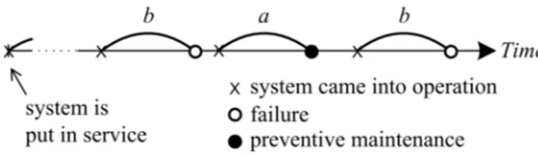
The notion of cycles is particularly important in our approach. Each measurement cycle is compounded by the condition measurements gathered from system operation start-up until stop, upon maintenance action. We call that the short-run horizon. On the other hand, we have the long-run horizon, which is composed by the measurement cycles cumulated over time. Fig. 3.2 presents a diagram which illustrates our approach.
Figure 3.2: The CBM approach proposed in this paper.
We start by performing the initial parameters estimation and we compute the optimal operating threshold based on this estimation. As time evolves, at each decision epochk, we have a condition measurement, which is used to estimate the system state, and an action is taken based on this estimation. Ifuk =S, we end a cycle carrying out a parameters re-estimation and a new
optimal threshold computation. k is reset to 0 and we start a new cycle.
3.2.1
Short-run and Long-run Optimization
As introduced in last paragraph, we consider a double time frame:
• Short-run horizon: from system start-up (k = 0) until system stop (uk =S).
• Long-run horizon: defined as the short-run horizons cumulated over time.
Chapter 3: A Model for Condition-Based Maintenance
Since we assume perfect repair (assumption 2, Section 3.2) by solving optimally the short-run model we also guarantee the long-run cost minimiza-tion. This is the subject of the following results.
Proposition 1(The structure of the long-run horizon problem). The optimal solution of the long-run horizon problem can be divided into various optimal sub-solutions, each sub-solution being the optimal solution of the associated short-run horizon problem.
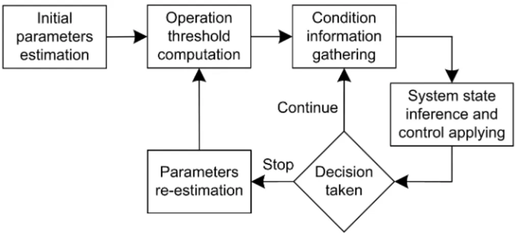
Proof. Under the assumption of perfect repair, we are able to slice the long-run horizon problem in various short-long-run horizon problems, all short-long-run problems having the same structure (however they might have different Ψ’s because of re-estimation step). Figure 3.3 illustrates that procedure. Notice that we reset k whenever a repair is carried out (uk=S). Thus, the system
is brought back to the state 1 (“as good as new”) and we set k = 0 at the same time the system operation restarts.
Figure 3.3: Long-run horizon optimization.
The Bellman’s Principle of Optimality states that “an optimal policy has the property that whatever the initial state and initial decision are, the remaining decisions must constitute an optimal policy with regard to the state resulting from the first decision” (Bellman, 1957). In other words, given an optimal sequence of decisions, each subsequence must also be optimal. The principle of optimality applies to a problem (not an algorithm) and a problem satisfying this principle has the so-called Optimal Substructure.
Chapter 3: A Model for Condition-Based Maintenance
Corollary 1 (Long-run horizon optimization). Solving optimally (cost min-imization) the short-run horizon implies in long-run optimization.
Proof. Since all short-run horizon problem (subproblems of the long-run hori-zon problem) have the same structure, by finding the solution of the short-run problem we get the long-run solution.
Alternative proof:
Let {µ1, µ2,· · · , µm,· · · } be the optimal policy for the long-run horizon
problem. Thenµmis the optimal policy of themth short-run horizon
(Propo-sition 1).
If µm was not an optimal policy of the mth short-run horizon, we could
then substitute it by the optimal policy for the mth short-run horizon, µ∗
m.
The result is a better policy for the long-run horizon problem. This contra-dicts our assumption that {µ1, µ2,· · · , µm,· · · }is the optimal policy for the
long-run horizon problem.
Thus, we focus the rest of the chapter on optimizing the short-run horizon.
3.3
Mathematical Formulation
Consider a multi-state deteriorating system subject to aging and sudden fail-ures, with states in deteriorating order from 1 (as good as new) to L (com-pletely failed) . If no action is taken the system is left as it is (uk =C). We
assume that the system condition evolution is a Markovian stochastic process and, since we consider periodic inspections, we can model the deterioration using a discrete-time Markov chain.
For this purpose, let {Xk}k≥0 be the Markov chain in question, where
Xk denotes the system condition at epoch k and {Xk} models the system
deterioration over time. The {Xk} state space is X ={1,2, . . . , L} with the
associated probability transition aij(uk=C), simply denoted as aij, defined
as
Chapter 3: A Model for Condition-Based Maintenance
aij = Pr[Xk+1=j|Xk=i, uk=C] = Pr[X1=j|X0=i, u0=C],
subject toPLj=iaij = 1, ∀i, j. For convenience, we express these probabilities
in matrix form: A≡[aij] .
Letg(·) be the cost of the system at each period, written as function of the system’s state (Xk) and the decision taken (uk). This function denotes the
expected operational system’s cost, the expected unavailability cost incurred upon failure and/or maintenance actions and the expected maintenance ac-tion costs themselves, as follows:
• For xk∈1, . . . , L−1 we have:
– uk =C(continue to operate, i.e., do nothing): g(xk, uk) represents
the operational system’s cost, which can be written in terms of the system’s state;
– uk = S (stop the operation and perform the preventive
main-tenance): g symbolizes the expected preventive maintenance cost (including the unavailability cost), which can be written as a func-tion of the system’s state: in general, the poorer the condifunc-tion the higher the cost;
• For xk=L (failed):
– uk = S: g(·) describes the expected corrective maintenance cost,
including the unavailability cost carried out during the repair;
– uk =C: g(·) represents the unavailability cost over period [k, k+1),
generally a non-optimal decision, since it implies that the system no longer operates.
Now we introduce the following definition:
Chapter 3: A Model for Condition-Based Maintenance
1. the system condition can be improved only by a maintenance interven-tion. That is, A entries can be written as
aij =
(
Pr[Xk+1=j|Xk=i, uk=C], if j ≥i,
0, otherwise. (3.1)
2. if no maintenance action is taken, there is a positive probability that the state L will be reached after p periods (L is reachable), i.e.,
Pr[Xp =L|X0 = 1] >0, with uk =C,∀k < p.
This condition, together with the first, implies that L is also an absorb-ing state if uk =C,∀k < p.
3. the unavailability cost incurred by the system non-operation is higher than the corrective maintenance cost, i.e.,
g(Xk =L, uk =C)> g(Xk=L, uk=S).
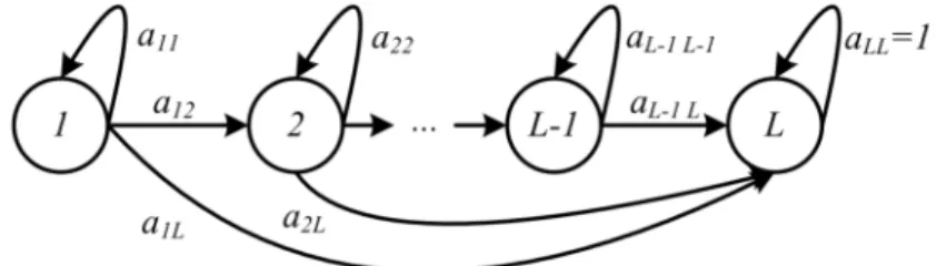
Fig. 3.4 illustrates the Markov chain of a well-defined problem. It reflects the wear out deterioration. Once the system is deteriorated, its condition cannot be improved over time (unless by a maintenance intervention). More-over, the probabilities aiL, ∀i ∈ {1, . . . , L−2}, denotes the sudden failure.
Hereafter, it is assumed that the problem is well-defined.
Figure 3.4: The Markov chain that denotes the system condition evolution (Xk). The probabilities aij:j>i+1,i<L have been omitted for succinctness.