Decision Science Letters 4 (2015) 465–476
Contents lists available at GrowingScience
Decision Science Letters
homepage: www.GrowingScience.com/dsl
Fuzzy goal programming applied to multi-objective programming problem with FREs as constraints
Kailash Lachhwani1*
Department of Applied Sciences, National Institute of Technical Teachers Training and Research, Chandigarh – 160 019, India
C H R O N I C L E A B S T R A C T
Article history:
Received February 9, 2015 Received in revised format: May 12, 2015
Accepted June 12, 2015 Available online June 15 2015
This paper presents an alternate technique based on fuzzy goal programming (FGP) approach to solve multi-objective programming problem with fuzzy relational equations (FREs) as constraints. The proposed technique is more efficient and requires less computational work than that of algorithm suggested by Jain and Lachhwani (2009) [Jain, & Lachhwani (2009). Multiobjective programming problem with fuzzy relational equations. International Journal of Operations Research, 6(2), 55−63.]. In FGP formulation, objectives are transformed into the fuzzy goals using maximum and minimal solutions elements of FREs feasible solution set. A pseudo code computer algorithm is developed for computation of maximum solution of FREs. Suitable linear membership function is defined for each objective function. Then achievement of the highest membership value of each of the fuzzy goals is formulated by minimizing the sum of negative deviational variables. The aim of this paper is to present a simple and efficient solution procedure to obtain compromise optimal solution of multiobjective optimization problem with FREs as constraints. A comparative analysis is also carried out between two methodologies based on numerical examples.
All rights reserved.
Growing Science Ltd. 5
© 201
Keywords:
Fuzzy relational equations Minimal solution
Compromise optimal solution Fuzzy goal programming
1. Introduction
Fuzzy relational equations (FREs) play an important role in fuzzy set theory and fuzzy logic systems, from both of the theoretical and practical view points. The importance of fuzzy relational equations is best described by Zadeh, the founder of fuzzy set theory in the foreword of monograph authored by Di Nola et al. (1989): “Human knowledge may be viewed as a collections of facts and rules, each of which may be represented as the assignment of a fuzzy relation to the unconditional or conditional possibility distribution of a variable. What this implies is that knowledge may be viewed as a system of fuzzy relational equations. In this perspective, then inference from a body of knowledge reduces to the solution of a system of fuzzy relational equations”. The initial works on fuzzy relational equations appeared in the beginning of 1970s., inspired by the applications of fuzzy relations in medical
1K. Lachhwani was earlier associated with Government Engineering College, Bikaner (Rajasthan) - 334 004, India
* Corresponding author. Tel. +91-0172-2759771, mob. +91-9214460018 E-mail address: [email protected] (K. Lachhwani) © 2015 Growing Science Ltd. All rights reserved.
diagnosis. Sanchez (1976) formulated some basic problems for fuzzy relational equations. Di Nola et al. (1989) presented a comprehensive overview of fuzzy relational equations in the first monograph on this issue. Some overviews can also be found in Di Nola et al (1991), Gottwald (1991, 1991a), Klir and Yaun (1995), Pedrycz (1991) and also Di Nola et al. (1984) for references.
As of today fuzzy relational equations have been intensively investigated from both the theoretical and practical view points and widely applied in decision making and optimization problems. Fang and Li (1999) studied the solution set of fuzzy relational equations with max product composition and an optimization problem with a linear objective function subject to such FREs. Sanchez’s work (1976) shed some light on this important subject. Since, then researchers have been trying to explain the problem and develop solution procedures. Lu and Fang (2001) used fuzzy relational equations constraints to study the non-linear optimization problems. Recently jain and Lachhwani (2009) suggested solution procedure of multiobjective programming problems with FREs constraints based on fuzzy mathematical programming. Mohamed (1997) introduced goal programming (GP) approach for multi decision making problems. Further, Pramanik and Roy (2007) extend it to solve multilevel programming problems (MLPPs). Baky (2009) proposed FGP algorithm for solving decentralized bi-level multiobjective (DBL –MOP) problems. Lachhwani (2012) suggested solution procedure for multiobjective quadratic programming problem based on fuzzy goal programming approach. Lachhwani and Poonia (2012) proposed FGP approach for multi-level linear fractional programming problem. Lachhwani (2013) described fuzzy goal programming approach for multi-level multiobjective linear programming problems. Abo-Sinna and Baky (2013) gave TOPSIS approach for multiobjective decision making problems. Thereafter, Lachhwani and Nehra (2014) suggested Modified FGP approach and MATLAB program for solving multi-level linear fractional programming problems. The aim of this paper is to apply FGP approach to multiobjective programming problem (MOPP) with FREs as constraints. Here we consider MOPP with FREs as constraints as:
max{Z x Z1( ), 2( ),...,x Zp( )}x
where
1
( ) m
l i i
i
Z x c x
=
=
∑
l =1, 2,…,psubject to (1)
, A x bο =
0≤ ≤xi 1
The membership matrices A, b, x are denoted by A=(aij),b=( ),bj x=( )xi where a b xij, j, i are real
numbers in the unit interval [0, 1] for all i∈I and j∈J. I={1, 2,..., }m and J ={1, 2,..., }n are the index sets. A system of FREs defined by A and b is denoted by
,
A x bο = (2)
where operator “ο” represents the max-min composition. The resolution of Eq. (2) is a set of solution vectorx ( , ,..., )= x x1 2 xm , 0≤ ≤xi 1, such that
min( ij, ) i i
j J
max a x b
∈
− = ∀ ∈i I (3)
Also cT =( ,c c1 2,...,cm)∈Rmbe an m-dimensional vector. Using the proposed methodology based on fuzzy goal programming approach, the problem (1) can be reduced to
min 1
p
l l
d
λ −
=
=
∑
subject to
( ) ( ) 1
l i l l l
Z Z x Z Z d−
− + + − ≥ l =1, 2,…,p (4)
,
A x bο =
This paper aims at presenting simple and efficient method for solving multiobjective optimization problem with FREs as constraints. The proposed method based on fuzzy goal programming approach is used to obtain compromise optimal solution by minimizing the sum of negative deviational variables in order to achieve highest value of each of fuzzy goals. The paper is organized as follows: In section 2, we discuss some basic properties of FRE’s solution sets, objective functions and other related facts in context of multiobjective programming problem. In next section, we derive proposed methodology based on FGP approach to obtain compromise optimal solution of problem. Detailed description of stepwise algorithm is given in section 4. Comparative analysis based on numerical example is discussed in section 5. Concluding remarks are given in section 6. Pseudo code computer algorithm is given in appendices at the end.
2. Properties of FRE’s solution sets and Objective functions
2.1 Characterization of feasible solution set of FREs
LetX A b( , ) be the complete set of solution. Then ifX A b( , )≠0, it can be determined by unique maximum solution and a finite number of minimal solutions suggested by Adamopoulos and Pappis (1993) as follows:
Lemma 1. For anyi∈I, ∃ some j∈J, such that aij≥bj, then X A b( , )≠φ.
Proof. Let X A b( , )=φ, then it will have no solution if max aij <bi for some i∈Ias by Klir and Yuan
(1995), contrary to this X A b( , )≠φ,if for any i∈I, ∃some j∈J such that aij≥bi.
Lemma 2. If x ( , )∈X A b then min(a xij, j)=bifor some j∈Jand min(a xij, j)≥bifor otherj∈J.
Proof. By Equation (3), max-min (a xij, j)=bi.This implies min(a xij, j)≤bi. Since x∈X A b( , ), therefore
there exists at least one j∈Jsuch that min(a xij, j)=bi. Now we should have following related definitions as:
Definition 1. xˆ∈X A b( , ) is called a maximum solution if x≤xˆ for all x∈X A b( , ). The minimum solution can be obtained as given by Chanas (1989):
1
ˆ @ ( @ )
m
j ij j
i
x A b a b j J
=
= = ∀ ∈
∧
(5)
where
1
( @ )
ij j
ij j
j ij j
if a b
a b
b if a b
≤
= >
(6)
and
min( , )
a∧ =b a b (7)
Also xˆ thus obtained is feasible if A x bο = , and Ji=
{
j a, ijοxˆj= ∀ ∈bi}
i I, where Ji is adjoin partition of I.Definition 2. Fang and Puthenpura (1993): Minimal solution: x∈X A b( , )is called minimal solution if
x≤xfor any x∈X A b( , )implies thatx=x. Denote the set of all minimal solutions byX A b( , ), the complete set of solutions X A b( , )is obtained by
{
}
( , )
ˆ ( , )
x X A b
X A b x X x x x
∈
= ∪ ∈ ≤ ≤ (8)
Step 1. Compute Ω using
, i 0
i
j J i I b
b j
∈
∈ ≠
Ω =
∏
∑
(9)Step 2. Now convert Ω into conjunctive normal form.
Step 3. For simplification of Ω
Using conjunctive operator
( , )
max
.
c d
l if l k
c d
l k unchanged if l k
=
= ≠
(10)
and using disjunctive operator
1 2
1 2 1 2
1 2
1 2 1 2
. .... , . .... . ... , m i i m m m m m c c c
if c d
c d
c c d d
l l l i I
l l l l l l
unchanged otherwise ≤ + = ∀ ∈ (11)
Step 4. Suppose Ωhas s step after the step 3, then X A b( , )has s elements which can be computed as:
( ) ( ) ( ) ( ) 1 2
(p p , p ,..., p )
n
x = x x x
(12)
where ( )p ( )p
j j
x =c , j∈J and p=1, 2,...,s
1.2 Characterization of Objective function
Here we characterize the objective function as suggested by Fang and Li (1999) in following manner:
{ T , ( , )}
Z= =z c x x∈X A b (13)
If cT ≥0, then the linear function z=cT xis monotonically increasing and positive say zand if cT ≤0 is
a monotonically decreasing and negative over X A b( , ) say z, then z= +z z. For any given
1 2
( , , ..., )
T n
n
c = c c c ∈R , we define ( ,1 2,..., )
T
n
c = c c c and ( ,1 2,..., )
T
n
c = c c c
such that
0
0 0
j j
j
j
c if c
c
if c
≥
= <
0 0
0 j j j j if c c
c if c
≥
= <
(14)
Obviously
T T T
c =c +c , thus for any x∈X A b( , ),z = z + zand hence maxz=maxz+maxz (15)
Lemma 3. If cj ≤ ∀ ∈0, j J,then max *
T
z = c x
.
Proof. Since x0≤ ≤x xˆand cT ≤0, therefore
0
ˆ
T T T
c x≤c x≤c x and *
x will be such that c xT *=max
{c xT ,x∈X A b( , )}, so max T *
z =c x
.
Lemma 4. If cj ≥ ∀ ∈0, j J , then maxz = c xTˆ.
Proof. ∀ ∈x X A b( , ), 0≤ ≤x xˆand c xTˆ≥c xT ,therefore maxz = c xTˆ.
Hence
maxz = max max z + z = c xTˆ + c xT *, (16)
where optimal solution *
{ j }
x = x j∈J is the combination of *
* *
ˆ 0
0
j j
j
j
x if c
x j J
x if c
<
= ∀ ∈
≥
(17)
3. Proposed FGP Methodology
For Multiobjective programming problem with FREs as constraints, Pareto optimal solution is required as a necessary condition in order to guarantee the relationality of decisions. However, In FGP approach compromise optimal solution may be treated as satisfactory solution in order to optimize multiple objectives. We need to express the definitions related to efficient solution and compromise optimal solution in context of multi-objective programming problem as:
Definition 3. Pareto Optimal Solution (Efficient Solution):x0∈X is an efficient solution to
multi-objective programming problem Eq.(1) if and only if there exists no otherx∈X such that 0
l l
Z ≥Z for
all l=1,2,…,p and 0
l l
Z >Z for at least one l.
Definition 4. Compromise Efficient Solution: For problem Eq. (1), a compromise efficient solution is an efficient solution selected by the decision maker (DM) as being the best solution where the selection is based on the DM’s explicit or implicit criteria.
Zeleny (1982) as well as most authors describes the act of finding a compromise solution to problem Equation (1) as “… an effort or emulate the ideal solution as closely as possible”.
In present methodology criteria selected by DM’s is based on minimizing the sum of negative deviational variables so that each fuzzy goal (membership function) can attain it’s as maximum value as possible subject to satisfying FREs. Hence for problem (1), a compromise obtained solution is pareto optimal solution selected by the decision makes (DM) as being the best solution when the decision is based on the DM’s Criteria.
Our FGP model for determining compromise optimal (efficient) solution based on the finding of the totality or subset of efficient solutions with the DM, then choosing one best solution on some explicit or implicit algorithm.
3.1 Fuzzy goal programming formulation of problem
To formulate the fuzzy goal programming model to problem (1), each objective function Z xl( ) ( 1, 2,...,
l= p) would be transformed into fuzzy goals by means of assigning their corresponding individual maximum values as an aspiration level to each of them. They are to be characterized by the associated membership functions.
3.1.1 Characterization of membership functions
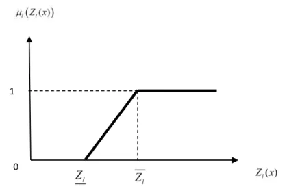
To build membership functions, fuzzy goals and their aspiration levels should be determined first. Using the individual best solution, we obtain maximum and minimum values of each objective functions and then construct membership function (as shown in figure 1), as the following:
1 ( )
( )
( ( )) ( )
0 ( )
l l
l l
l l l l l
l l
l l
for Z x Z Z x Z
Z x for Z Z x Z
Z Z
for Z x Z
µ
≥
−
= ≤ ≤
−
≤
∀ =l 1, 2,...,p (18)
Fig. 1. Membership function for µl
(
Z xl( ))
l=1, 2,...,p3.2FGP Solution Approach
Fuzzy goal programming (FGP) is an extension of conventional goal programming (GP) introduced by Charnes and Cooper (1962). GP has been extensively studied and widely circulated in literature. In this paper, GP approach to fuzzy multi-objective decision making problems introduced by Mohamed (1997) is extended to solve MOPPs with FREs as constraints problems. In decision making situation, the aim of each DM is to achieve highest membership value (unity) of the associated fuzzy goal in order to obtain the absolute satisfactory solution. However, in real practice, achievement of all membership values to the highest degree (unity) is not possible due to conflicting nature of objectives. Therefore, decision policy for minimizing the regrets of the decision makers (DMs) for all objectives should be taken into consideration. Then each DM should try to maximize his or her membership function by making them as close as possible to unity by minimizing its negative deviational variables. Therefore, in effect, we are simultaneously optimizing all the objective functions. So, for the membership functions defined in Eq. (18), the flexible membership goals having the aspired level unity can be represented as:
( ( )) 1
l Z xl dl dl
µ + −− + =
1, 2,..., ,
l= p (19)
where dl ,dl ( 0)
− + ≥ (
1, 2,..., )
l= p represent the under and over deviational variables respectively from the aspired levels. In conventional GP, the under and/or over deviational variables are included in the achievement function for minimizing them and that depends upon the type of objective functions to be optimized. Thus MOPP problem (1) changes into
min
1
p
l l
d
λ −
=
=
∑
subject to
( ) ( )( ) 0
l i l l l l
Z Z x Z Z d− d+
− + + − − = l =1, 2,…,k (20)
,
A x bο =
0≤ ≤xi 1
In this FGP approach, only the sum of under deviational variables is required to be minimized to achieve the aspired level. It may be noted that any over deviational from a fuzzy goal indicate the full achievement of the membership value. Now it can be easily realized that the membership goals in Eq. (19) are inherently linear equations and this may reduce computational difficulties in the solution process. However, for model simplification the Eq. (19) can be considered as a general form of goal
1
expression of the above stated membership goals. It may be noted that when a membership goal is fully achieved, negative deviational variable become zero and when its achievement is zero, negative deviational variable become unity in the solution. Now if the most widely used and simplest version of GP (i.e. minsum GP) is introduced to formulate the model of the problem under consideration, the GP model formulation becomes:
(FGP Model) min
1
p
l l
d
λ −
=
=
∑
subject to
( ) ( ) 0
l i l l l
Z Z x Z Z d−
− + + − ≥ l =1, 2,…,p (21)
,
A x bο =
0≤ ≤xi 1
4. Algorithm
In this section, stepwise algorithm of proposed methodology can be described as follows:
Step 1. Compute
1
ˆ ( @ ),
m
j ij i
i
x a b j J
=
=
∧
∀ ∈ according to Equation (7) and construct maximum solutionˆx.The pseudo code computer algorithm is developed for this step and is given in appendices. Using this code, computer program can be constructed to obtain maximum solution xˆ=( , ,..., )x xˆ ˆ1 2 xˆn ∈X A bˆ( , ).
Step 2. Check the feasibility A x bο = ,if yes, go to next step, otherwise stop and the problem has no solution.
Step 3. Find the index set Ji ={j∈J aijοxj =bi}, .∀ ∈i I
Step 4. Find the minimal solution setX A b( , )as given in section 3.
Step 5. Define average cost vector T c and T
c
according to (14).
Step 6. Compute zl =c xTl ˆ,∀ =l 1, 2, ...,p and
T
l l
z =c x
for all minimal solutions.
Step 7. Calculate for all minimal solutionsZl = +z l zl.
Step 8. Compute Zl = +z l zlfor maximumzland Zl = +z l zlfor minimumzl.
Step 9. Put the values in Eq. (21), and solve the reduced problem
min
1
p
l l
d
λ −
=
=
∑
subject to
( ) ( ) 1
l l l l l
Z Z x Z Z d−
− + + − ≥ l =1, 2,…,p (22)
,
A x bο =
0≤ ≤xi 1
5. Numerical example
Illustration 1. Consider the following MOPP with FREs constraints as:
max
{
Z x Z x Z x1( ), 2( ), 3( )}
where 1( ) 1
T
Z x =c x, 2( ) 2
T
Z x =c x, 3( ) 3
T
Z x =c x
subject to
, A x bο = 0≤ ≤xi 1
where
0.5 0.8 0.9 0.3 0.85 0.4
0.2 0.2 0.1 0.95 0.1 0.8
0.8 0.8 0.4 0.1 0.1 0.1
0.1 0.1 0.1 0.1 0.1 0.1
A =
with m=4and n=6 1 (3, 4,1,1, 1, 5),
T
C = − 2 (1,1,1,1, 1,1),
T
C = − 3 (1, 2, 3, 4, 1, 5),
T
C = − (.85, 0.6, 0.5, 0.1)T
b= .
Step 1. For the above given A and b , using constructed pseudo computer algorithm given in appendices, we find: xˆ=A@b =(0.5, 0.5, 0.85, 0.6,1.0, 0.6).
Step 2. xˆ is feasible, since A xο =ˆ b. Thus A xο =ˆ b
Step 3. For I=
{
1, 2, 3, 4 ,}
J1 ={ }
3, 5 , J2 ={ }
4, 6 , J3={ }
1, 2 , J4={
1, 2, 3, 4, 5, 6}
Step 4. s=8 and the minimal solutions are (1)
(0.0, 0.5, 0.0, 0.0, 0.85, 0.6)
x = ,
(2)
(0.0, 0.5, 0.0, 0.6, 0.85, 0.0)
x = , (3)
(0.0, 0.5, 0.85, 0.0, 0.0, 0.6)
x =
, (4)
(0.0, 0.5, 0.85, 0.6, 0.0, 0.0)
x = ,
(5)
(0.5, 0.0, 0.0, 0.0, 0.85, 0.6)
x = , (6)
(0.5, 0.0, 0.0, 0.6, 0.85, 0.0)
x = , (7)
(0.5, 0.0, 0.85, 0.0, 0.0, 0.6)
x = ,
(8)
(0.5, 0.0, 0.85, 0.6, 0.0, 0.0)
x = .
Step 5. 1 (3, 4,1,1, 0, 5)
T
c = and 1 (0, 0, 0, 0, 1, 0)
T
c = −
; 2 (1,1,1,1, 0,1)
T
c = and 2 (0, 0, 0, 0, 1, 0)
T
c = −
; 3 (1, 2, 3, 4, 0, 5)
T
c = and
3 (0, 0, 0, 0, 1, 0)
T
c = −
.
Step 6. 1 1 ˆ 7.95
T
z =c x = ; 2 2ˆ 3.05
T
z =c x = ; 3 3 ˆ 8.40
T
z =c x = . For all minimal solutions (computed in step 4), the values of 1 1
T z =c x
are -0.85, -0.85, 0.0, 0.0, -0.85, -0.85, 0.0, 0.0., the values of 2 2
T z =c x
are
-0.85, -0.85, 0.0, 0.0, -0.85, -0.85, 0.0, 0.0 and the values of 3 3T z =c x
are -0.85, -0.85, 0.0, 0.0, -0.85, -0.85, 0.0, 0.0.
respectively.
Step 7. The values of objective functions z1= +z 1 z1,z2 =z 2+z2 and z3=z 3+z3with corresponding solutions respectively are
(1)
1 2 3
* (0.5,0.5,0.85,0.6,0.85,0.6), 7.10, 2.20, 7.55
x = z = z = z = x*(2)=(0.5,0.5,0.85,0.6,0.85,0.6),z1=7.10, 2.20, 7.55z2= z3= (3)
1 2 3
* (0.5,0.5,0.85,0.6,0.0,0.6), 7.95, 3.05, 8.40
x = z = z = z = x*(4)=(0.5,0.5,0.85,0.6,0.0,0.6),z1=7.95,z2=3.05, 8.40z3= (5)
1 2 3
* (0.5,0.5,0.85,0.6,0.85,0.6), 7.10, 2.20, 7.55
x = z = z = z = (6)
1 2 3
* (0.5,0.5,0.85,0.6,0.85,0.6), 7.10, 2.20, 7.55
x = z = z = z =
(7)
1 2 3
* (0.5,0.5,0.85,0.6,0.0,0.6), 7.95, 3.05, 8.40
x = z = z = z = (8)
1 2 3
* (0.5,0.5,0.85,0.6,0.0,0.6), 7.95, 3.05, 8.40
x = z = z = z =
Step 8. max( )z1 = 7.95;z1= max( )z2 = 3.05;z2 = max( )z3 = 8.40z3 = ; max( )z1 = 7.10;z1 =
2 2
min( )z = 2.20;z =
min( )z3 = 7.55z3 =
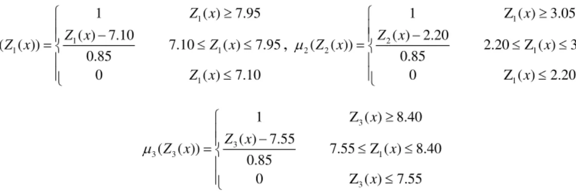
1
1
1 1 1
1
1 ( ) 7.95
( ) 7.10
( ( )) 7.10 ( ) 7.95
0.85
0 ( ) 7.10
Z x Z x
Z x Z x
Z x µ ≥ − = ≤ ≤ ≤ , 1 2
2 2 1
1
1 Z ( ) 3.05
( ) 2.20
( ( )) 2.20 Z ( ) 3.05
0.85
0 Z ( ) 2.20
x Z x
Z x x
x µ ≥ − = ≤ ≤ ≤ 3 3
3 3 1
3
1 Z ( ) 8.40
( ) 7.55
( ( )) 7.55 Z ( ) 8.40
0.85
0 Z ( ) 7.55
x Z x
Z x x
x µ ≥ − = ≤ ≤ ≤
Step 10. Using the proposed FGP model as given in Eq. (20), the problem reduces to
minλ d1 d2 d3
− − −
= + +
subject to
1 2 3 4 5 6 1
3x +4x + +x x -x +5x +0.85d− ≥7.10
1 2 3 4- 5 6 0.85 2 2.10
x +x +x +x x +x + d−≥
1 2 2 3 3 4 4- 5 5 6 0.85 3 7.55
x + x + x + x x + x + d−≥
Aο =x b
0
x≥
Solving this L.P.P, the compromise solution of MOLPP is (3) (4) (7) (8)
* * , * , * , *
x =x x x x
(0.5, 0.5, 0.85, 0.6, 0.0, 0.6)
= with values z1=7.95, z2 =3.05 and z3 =8.40withλ =0.52941. Also the values of
membership functions achieved are:µ1(Z x1( ))=1, µ2(Z x2( ))=1, µ3(Z x3( ))=1. Note that using technique suggested by Jain and Lachhwani (2009) for solution of above problem, the compromise optimal solution of this problem thus will be: (3) (4) (7) (8)
* * , * , * , *
x =x x x x =(0.5, 0.5, 0.85, 0.6, 0.0, 0.6),with values
1 7.95,
z = z2 =3.05 andz3=8.40. Also the values of membership functions achieved are: µ1(Z x1( ))=0,
2(Z x2( )) 0
µ = ,µ3(Z x3( ))=0.
Illustration 2. Consider the following MOPP with FREs constraints as:
max
{
Z x Z x1( ), 2( )}
where 1( ) 1
T
Z x =c x, 2( ) 2
T
Z x =c x
subject to ,
A x bο =
0≤ ≤xi 1
with
0.5 0.8 0.9 0.3 0.85 0.4
0.2 0.2 0.1 0.95 0.1 0.8
0.8 0.8 0.4 0.1 0.1 0.1
0.1 0.1 0.1 0.1 0.1 0.1
A =
and m=4, n=6 1 (3, 4,1,1, 1, 5),
T
C = − 2 (1,1,1,1, 1,1),
T
C = − (.85, 0.6, 0.5, 0.1)T
b=
Using the proposed methodology, the problem reduces to minλ d1 d2
− −
= +
subject to
1 2 3 4 5 6 1
3x +4x + +x x -x +5x +0.85d− ≥7.10
1 2 3 4- 5 6 0.85 2 2.10
x +x +x +x x +x + d−≥
Aο =x b
0
Solving this L.P.P, the compromise solution of MOLPP is (3) (4) (7) (8)
* * , * , * , *
x =x x x x
(0.5, 0.5, 0.85, 0.6, 0.0, 0.6)
= with values z1=7.95 and z2 =3.05. .Also the values of membership functions
achieved are:µ1(Z x1( ))=1,µ2(Z x2( ))=1, µ3(Z x3( ))=1.
Note that using technique suggested by Jain and Lachhwani (2009) for solution of above problem, the compromise optimal solution of this problem thus will be: (3) (4) (7) (8)
* * , * , * , *
x =x x x x
(0.5, 0.5, 0.85, 0.6, 0.0, 0.6)
= with values z1=7.95andz2 =3.05. Also the values of membership functions achieved are:µ1(Z x1( ))=0,µ2(Z x2( ))=0, µ3(Z x3( ))=0.
Comparison tables (table 1 and table 2) show that the proposed FGP approach is more efficient than technique suggested by Jain and Lachhwani (2009) in context of achieving values of membership functions. Also the proposed FGP approach requires less computational works as compared to the technique suggested by Jain and Lachhwani (2009) because the proposed technique does not require to
compute the distance function ( ) 2 ( )1/ 2
{ }
l l
l
lj
Z Z x
d x
c
− =
∑
and p=Sup d { }l ∀ = l 1, 2,...,p. This reduces lots ofcomputational works in proposed FGP approach.
Table 1
Comparison of membership function values for example 1
Proposed FGP approach Solution technique by Jain and Lachhwani (2009)
z1 = 7.95, μ1(z1) = 1 z1 = 7.95, μ1(z1) = 0
z2 = 3.05, μ2(z2) = 1 z2 = 3.05, μ2(z2) = 0
z3 = 8.40, μ3(z3) = 1 z3 = 8.40, μ1(z1) = 0
Table 2
Comparison of membership function values for example 2
Proposed FGP approach Solution technique by Jain and Lachhwani (2009)
z1 = 7.95, μ1(z1) = 1 z1 = 7.95, μ1(z1) = 0
z2 = 3.05, μ2(z2) = 1 z2 = 3.05, μ2(z2) = 0
6. Conclusions
An effort has been made to apply fuzzy goal programming approach to solve multiobjective programming problem with FRE’s as constraints to obtain the compromise optimal solution using proposed methodology which is more efficient and requires less computational work as compared to the earlier technique. The main difficulty with the proposed methodology is to obtain feasible solution set of FRE’s. However, this computational work can be reduced using computer algorithm. Also the complexity in equations can be reduced using stepwise procedure for finding out all minimal solutions for the given system of FRE’s.
Acknowledgements
The Author would like to thank the anonymous reviewers for their valuable comments and suggestions to improve the quality and presentation of this paper. Author is also thankful to the authorities of institution Government Engineering Colllege Bikaner (Rajasthan, India) for providing necessary facilities where this work was partially carried out.
References
Adamopoulos, G. I. & Pappis, C. P. (1993). Some results on resolution ring the present Investigation in this revised form of fuzzy relation equations. Fuzzy Sets and System, 60(1), 83-88.
Baky, I.A., & Abo-Sinna, M.A. (2013). TOPSIS for bi-level MODM problems. Applied Mathematical Modelling, 37, 1004–1015
Chanas, S. (1989). Fuzzy programming in multiobjective linear programming: a parametric approach.
Fuzzy Sets and Systems, 29, 303-313.
Charnes, A. & Cooper, W. W. (1962). Programming with linear fractional functional. Novel Research Logistics Quarterly, 9, 181-186.
Fang, S. C., & Li, G. (1999). Solving fuzzy relation equations with a linear objective function. Fuzzy Sets and Systems, 103, 107-113.
Fang, S. C., & Puthenpura, S. (1993). Linear optimization and extensions: theory and algorithm. Prentice –Hall, Englewood Cliffs, NJ.
Gottwald, S. (1999). Approximately solving fuzzy relational equations: Some mathematical results and some heuristic proposals. Fuzzy Sets and Systems, 66, 175-193.
Gottwald, S. (1999). Approximate solutions of fuzzy relational equations and Characterization of t – norms that defines for fuzzy sets. Fuzzy Sets and Systems, 75, 189 – 201.
Jain, S., & Lachhwani, K. (2009). Multiobjective programming problem with fuzzy relational equations. International Journal of Operations Research, 6(2), 55-63.
Klir, G. J., & Yuan, B. (1995). Fuzzy sets and fuzzy logic: theory and applications. Prentice- Hall, PTR, USA.
Lu, J., & Fang, S. C. (2001). Solving nonlinear optimization problems with fuzzy relation equations constraints. Fuzzy Sets and Systems, 119, 1-20.
Lachhwani, K. (2009). Fuzzy goal programming approach to multi-objective quadratic programming problem. Proceeding of National Academy of Sciences India, 82(4), 317-322.
Lachhwani, K., & Poonia, M. P. (2012). Mathematical solution of multilevel fractional programming
problem with fuzzy goal programming approach. Journal of Industrial Engineering
International, 8(1), 1-11.
Lachhwani, K. (2013). On solving multi-level multi objective linear programming problems through fuzzy goal programming approach. OPSEARCH, 51 (4), 624-637.
Lachhwani, K., & Nehra, S. (2014). Modified FGP approach and MATLAB program for solving multi-level linear fractional programming problems. Journal of Industrial Engineering International,
11(1), 15-36.
Mohamed, R. H. (1997). The relationship between goal programming and fuzzy programming. Fuzzy Sets and Systems, 89, 215-222.
Nola, A. D., Sessa, S., Pedrycz, W., & Sanchez, E. (1989). Fuzzy relational equations and their applications in knowledge engineering. Kluwer Academic Publishers, Dordrecht.
Nola, A. D., Pedrycz, W., & Sessa, S. (1984). Some theoretical aspects fuzzy relational equations describing fuzzy system. Information Sciences, 34, 261-264.
Nola, A. D., Pedrycz, W., Sessa, S., & Sanchez, E. (1991). Fuzzy relation equations theory as a basis
of fuzzy modeling: an overview. Fuzzy Sets and Systems, 40, 415-429.
Pramanik, S., & Roy, T. K. (2007). Fuzzy goal programming approach to multi level programming problems. European Journal of Operational Research, 176, 1151-1166.
Pedrycz, W. (1991). Processing in relational structures: fuzzy relational equational structures. Fuzzy Sets and Systems, 25, 77-106.
Sanchez, E. (1976). Resolution of composite fuzzy relation equations. Information and Control, 30, 38-48.
Appendices
The pseudo code computer algorithm for the step 1 can be given as: // M is the number of rows of matrix, N is the number of columns.
// A(10) (10) is the two dimensional matrix with 10 rows and 10 columns. // B (10) is the one dimensional matrix with 10 elements.
// C (10) is the one dimensional matrix with 10 elements. //X (10) is the one dimensional matrix with 10 elements. // M, N, I, J are integer data types.
INPUT M INPUT N
REM DEFINE MATRIXES DIM A (M, N)
DIM B (M) DIM C (M)
REM READ A MATRIX FOR I = 1 TO M
FOR J = 1 TO N INPUT A (I, J) NEXT J NEXT I
REM READ B MATRIX FOR I = 1 TO M
INPUT B (I) NEXT I
FOR J = 1 TO N FOR I = 1 TO M
IF A (I) (J) <= B (I) THEN LET X (I) = 1
NEXT I NEXT J ELSE
LET X (I) = B (I) END IF
LET C (J) = X (0) FOR I = 1 TO M IF C (J) > X (I) THEN C (J) = X (I)
NEXT I END IF
REM OUTPUT RESULT FOR J = 1 to N
PRINT The Answer Matrix is following PRINT C (J)