Forecasting Inflation under Globalization with Artificial Neural Network-Based Thin and Thick Models

Forecasting Inflation under Globalization with

Artificial Neural Network-Based Thin and Thick

Models

∗

Tsui-Fang Hu

_{Iker Gondra Luja}

_{H. C. Su}

_{Chin-Chih Chang}

Abstract—We study globalization influences on forecasting inflation in an aggregate perspective us-ing the Phillips curve for Hong Kong, Japan, Taiwan and the US by artificial neural network-based thin and thick models. Our empirical results support the hypothesis that globalization influences do generate the downward tendency in inflation through time in all cases with different levels. Moreover, the artificial neural network-based thin and thick models that have been developed upon the best linear model for each country have shown significant superiority over the naive model in the most cases and over the best lin-ear model in some cases. Finding optimal values of all the parameters for so many artificial neural network models is a difficult task because of the large number of parameters involved. Thus we do not make any claim on the optimality of the artificial neural network models in this study. As a consequence, even though our empirical results are not overwhelmingly satis-factory, building the artificial neural network model based upon the best linear model is a good compro-mise between practicality and optimality.

Keywords: artificial neural networks, nonlinearity, thick model

1

Introduction

Inflation is widely taken as one of the main economic problems, because it involves in the allocation efficiency of the economy by means of changing the relative prices among commodities. A dramatic acceleration of inflation results in large costs to the public and business commu-nity. The mechanism of how the relative-price adjust-ments among commodities affect (or cost) the economy is very complicated and not yet well understood. Pur-suing stable prices is the primary goal of a central bank

∗_{Manuscript received July 22, 2007.}

†_{P.O. Box 2166, State University, Arkansas 72467, USA}

Email: [email protected]

‡_{Department of Mathematics, Statistics & Computer Science,}

St. Francis Xavier University, Antigonish, NS B2G 2W5, Canada Email: [email protected]

§_{Department of Computer Science, Arkansas State University,}

State University, Arkansas 72467, USA Email: [email protected]

¶_{Department of Computer Science and Information}

Engi-neering, Chung Hua University, Hsinchu City 30012, Taiwan Email: [email protected]

while creating and maintaining an independent and ef-ficient monetary system. However, the acceleration in the pace of international trade in good, service and fi-nancial assets relative to the growth rate of the domestic trade, broadly defined as globalization, has attracted a lot of attentions [1]. This is because globalization has broken some macro rules such as a decrease in the corre-lations between the labor cost and inflation and a decline in the elasticities between import prices and core infla-tion. During the past decade, the acceleration in the pace of the world trade growth is well above the accel-eration in the pace of the world economic growth with a disparity from 2.99 percent in 1990 to 3.16 percent in 2006, specially in recent years, but the annual inflation in the advanced countries has been decreasing since 1990 and it is even well below the world economic growth rate. In other words, strong economic growth does not result in high inflation in the most advanced economies since 1990. Even for the developing countries, the annual in-flation has started to decelerate since 1995. The global trade (exports and imports of goods and services) stood 38 percent of the total world GDP in 1990 and hit 61 per-cent in 2006. Hence, it is hard to consider the domestic factors only while conducting the monetary policy when the domestic commodity and financial markets becomes increasingly open (and integrated to the world markets). As a result, globalization seems to become more and more important to this issue.

unemployment (NAIRU) can not provide more accurate forecasts than the naive forecasts. Therefore, to a cer-tain extent, the modern Phillips curve-based models are not as useful as expected. However, based on the study of McNelis and McAdam [6], the trimmed ANN-based thick model [9] outperforms the linear model for real-time and bootstrap forecasts in the Euro area as well as in some other countries considered in their study using the Phillips-Curve framework. Basically, they remove the 5

percent largest and smallest forecasts from several ANNs, and then use the average of the remaining forecasts as combined forecasts. It is practical to use a thick model on several neural networks in the first several forecasting periods, because there is no theoretical basis to select the best ANN among many ANNs that have different num-bers of neurons in the hidden layer, or different network architectures, but have same input variables. Even after some periods of forecasting, the forecasting performances of different ANNs might be still too close to determine which one is the best. Therefore a thick model can be ac-cordingly applied. However, the removals of the largest and smallest forecasts from several ANNs do not guaran-tee the best forecasting performance, insomuch as either the largest or the smallest forecast does not necessarily generate the largest forecasting error. To a certain ex-tent, the range for forecasts should be known a priori when using the trimming method. Moreover, an ANN-based thick (ANN thick) model might not always be a better choice over an ANN-based thin (single ANN; ANN thin) model, so we should consider the ANN thin model as well. Besides, the globalization factor, an increasingly important factor, is absent in their study.

The contribution of this paper is two-fold. First, we con-sider globalization influences while forecasting inflation in an aggregate perspective using the Phillips curve by artificial neural network-based thin and thick models for Hong Kong, Japan, Taiwan and the US that have data available for the globalization factor. Second, we compare the forecasting performances of ANN thin and thick mod-els with the forecasting performances of a simple naive and the best linear models. The paper is organized as follows. Section 2 describes the theoretical underpinnings and methodology. In Section 3, we discuss and compare the empirical results. The paper ends with some conclud-ing remarks.

2

Methodology

2.1 Theoretical Underpinnings of Artificial Neural Networks

Artificial Neural Networks (ANNs) are one of the most frequently used techniques in the field of machine learn-ing. The field of machine learning focuses on the study of algorithms that improve their performance at some task automatically through experience [10].

Suppose we are given training data as a set of n ob-servations. Each observation is a pair (x_i, y_i) where x_i ∈ ℜd and y_i ∈ ℜ. Assume that the training data

has been drawn independently from some unknown cu-mulative probability distributionP(x, y). The goal is to

find a functionf :ℜd_{→ ℜ that implements the optimal}

mapping. In order to make learning feasible, we have to specify a function spaceF from which the function is to be chosen. In particular, a set ofnpairs of training data, denoted by{(x_i, y_i)}n₁ , are given for the purpose of a

bi-nary classification task, wherex_i ∈ ℜd andy_i∈ {1,−1}

is the class label. Assume that the data is linearly sep-arable and letF be the set of linear decision boundaries of the form

f(x) =sign(w·x+b)

wherew∈ ℜd and b∈ ℜare the adjustable parameters.

Thus, choosing particular values forw and b results in

a trained classifier. For any trained classifier, the hy-perplane corresponding to w·x+b = 0 is the decision

boundary. A linear decision boundary is a simple classi-fier that can be learned very efficiently. However, due to its small complexity it can correctly classify data that is linearly separable only.

In general, one way to measure the performance of a trained classifier f ∈ F is to look at the mean error computed from the training data. This is known as the empirical risk (or training error). Minimizing the empirical risk is one of the most commonly used opti-mization procedures. However, even when there is no error on the training data, the classifier may not gener-ate correct classifications on unseen data (See Figure 1). This problem is known as overfitting. The ability of a classifier to correctly classify new data that is not in the training set is known as generalization. Having a classifier with good generalization is, of course, a much harder problem. There is a competition of terms. As the complexity of the classifier increases, the empirical risk tends to decrease. However, the generalization er-ror usually increases with increasing complexity. Thus, for such models with broad approximation abilities and few specific assumptions (e.g., ANNs), the distinction be-tween memorization and generalization becomes impor-tant [11]. A validation set (disjoint from the training set) is commonly used to assess generalization performance. Cross-validation is a technique that reduces overfitting. For instance, in a κ-fold cross-validation, the collected data is divided intoκ partitions. Each partition in turn is left out and the remaining κ−1 partitions are used for training. The left out partition is then used to test generalization performance. The value reported is then the average of theκtests.

(a) (b)

Figure 1: Generalization performance: a) an overly com-plex classifier that results in zero error on the training data, but may not generalize well to unseen data; b) a classifier that might represent the optimal tradeoff be-tween error in the classification of training data and com-plexity of the classifier, thus capable of generalizing well on unseen data.

elements (known as nodes or neurons) based on neurobio-logical models of the brain. One of their main advantages in comparison to other models is that they have very few domain-specific assumptions and are highly adapt-able (e.g., they learn from experience). Thus, they need no a priori assumption of a model and are capable of in-ferring complex non-linear input-output transformations. In addition to their typical use in (nonlinear) regression, they are commonly used in pattern recognition, where the ANNs assign a set of input features to one or more classes.

In the late 1950s, Rosenblatt [12] introduced the percep-tron learning rule, the first iterative algorithm for train-ing a simple ANN: the perceptron (see Figure 2), which is a linear classifier. After initializingwandbrandomly,

each training pointx_i is presented and the output value

ofyis compared againstyi. Ifyandyiare different (i.e., x_i is misclassified) the values ofwandb are adapted by

moving them either towards or away from x_i.

Rosen-blatt proved that, assuming the classes are linearly sepa-rable, the algorithm will always converge and find values for w and b that solve the classification problem. That

is, the algorithm finds a hyperplane that divides the d -dimensional space into two decision regions. A linear de-cision boundary (e.g., a single-layer perceptron) is a sim-ple classifier that can be learned very efficiently. However, due to its small complexity it can correctly classify data that is linearly separable only. On the other hand, a more complex decision boundary can correctly classify general data that may not be linearly separable.

The key idea responsible for the power, potential, and popularity of ANNs is the insertion of one or more lay-ers of nonlinear hidden units (between the inputs and output) [11]. These kinds of nonlinearity allow for inter-actions between the inputs (e.g., products between input variables). As a result, the network can fit more compli-cated functions [11]. A multilayer perceptron consists of

¦

x2

xd

w1

y w2

wd

b

1

Figure 2: One neuron single-layer d-input perceptron with threshold activation function. The output y =

sign(w·x+b) =sign(w_ix_i+b)

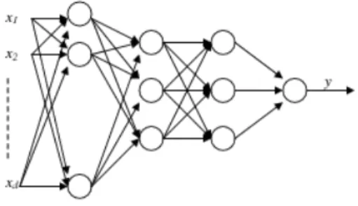
an input layer, at least one middle or hidden layer, and an output layer of computational neurons (see Figure 3). The input signals are propagated in a forward direction on a layer-by-layer basis.

Figure 3: Multilayerd-input perceptron with two hidden layers.

Learning in a multilayer network is similar to learning with a perceptron. That is, each training pointx_iis

pre-sented to the network as input. The network computes the corresponding output y. If y and yi are different,

the error is propagated. The sum of squared errors (over all training data) is the performance measure that the backpropagation algorithm attempts to minimize. When the value of this measure in an entire pass through all training data is sufficiently small, it is considered that the network has converged. The following section is go-ing to present the ANN models, inflation function, and data.

2.2 ANN thin and thick Models, Inflation Function, and Data

In contrast to traditional models that are “theory-rich” and “data-poor”, ANNs are “data-rich” and “theory-poor” in a way that little or no a priori knowledge of the problem is present [11]. Thus, they need no a priori assumption of a model and are capable of inferring complex non-linear input-output transformations. In spite of its easy ap-plication, there is no theoretical basis to select the best ANN among several ANNs that have different parameter values such as the numbers of neurons in the hidden layer (different network architectures) at the beginning of fore-casting periods, although they may have same input vari-ables. Moreover, the following situation could also pos-sibly occur: ANNs have no significant difference in their out-of-sample forecasting performances after a period of time. Usually there is a method, called thick model, that could be used under these circumstances. A thick model combines several forecasts from different ANNs. In the combination of several forecasts, the weights for the fore-casts can be equal or different. Alternatively, we can trim the outliers from the forecasts if we have prior informa-tion about the reasonable range of forecasts. Therefore, it is reasonable to use a thick model on several neural net-works in the first several periods of forecasting or when it is still hard to decide which ANN is the best after some periods.

In our study, ANN thin and ANN thick models are both considered. For the ANN thick model, we implement two different kinds. One is ANN thick with equal weight (i.e., average value) model, and the other one is ANN thick with unequal weight model that gives greater weight to the relatively better ANNs and less weight to the rela-tively worse ANNs by nonlinearly optimizing (minimiz-ing) the forecast error statistics from the first several out-of-sample test periods. In this study, we repeatedly esti-mate and update both the linear and several ANN models to obtain a one-step-ahead forecast (the real time fore-cast) while the sample period rolls forward a quarter at a time. For the purpose of avoiding obsolete information, we keep the sample size fixed by getting rid of the old-est data while the old-estimation is rolling over to the next period.

The Phillips curve framework with a globalization factor can be described as the following function for both the

linear and ANN models.

π4 t+1−π

4

t = f(∆π

4 t, ...,∆π

4

t−i,∆πt, ...,∆πt−j,

∆ut, ...,∆ut−m,∆gt, ...,∆gt−n)

whereπ4

t is the the 4-quarter change consumer price

in-dex (CPI) between quarters t and t−4 in an aggre-gate perspective at an annualized value as measured by

100[ln(Pt)−ln(Pt−4)], πt is quarterly inflation as

mea-sured by400[ln(Pt)−ln(Pt−1)], ut is the quarterly

em-ployment rate in quartert,gt is the quarterly

globaliza-tion factor (the ratio of exports plus imports to the overall GDP for a country) in quartert, andi, m,andnare the lag lengths. The left side term is the difference between the 4-quarter change inflation in the current quarter and the next quarter. We have to avoid forecasting long hori-zons such as the difference between the inflation over the next 4 quarters and inflation over the previous 4 quar-ters, although some research does not avoid forecasting long horizons [8, 6]. The reason is that a long forecasting horizon does not cohere with the Phillips curve theory that only exists in the short or medium run. In other words, there is no permanent tradeoff between inflation and unemployment in the long run, because the long-run inflation is determined by the central bank, i.e., the re-lationship in the Phillips cure does not exist in the long run. In addition, we also try different forms of informa-tion from the past such as the 4-quarter change employ-ment rate and 4-quarter change globalization factor to check if they also generate significant influences on ∆π4 t

in each country. As a result, only the 4-quarter change globalization factor is more significant than the quarterly globalization factor in the case of the US.

3

Empirical Results and Analysis

As mentioned previously, we repeatedly estimate and up-date both the linear and several neural network mod-els to get a one-step-ahead forecast (the real time fore-cast) from these different forecasting models. Since the economy evolves through time, it is not appropriate to keep obsolete information in our forecasting models, so we get rid of the earliest period while the estimation is rolling over to the next period. Thus, the sample size is fixed. The derived benefit to do so is that we can exam-ine the model’s evolution (model stability) through time, insomuch as it is not quite appropriate to use the same model while repeatedly estimating the forecasting models for a growing economy. As a result, the explainable vari-ables in each period might be different through time, and we can also obtain the time-varying coefficients for every input in the linear model and their relative importance through time. The linear model is a multivariate time se-ries model. To ensure that the residuals from the linear models are white noise, we perform the Breusch-Godfrey Lagrange multiplier test, Ljung-Box Q-statistics and cor-relogram of squared residuals while building the linear model in each period. Selecting the variables for the ANN models is based on the best linear model. The reason is that it is a very time-consuming and complex process to obtain all the optimal parameters (e.g., learning rate, number of neurons in each layer, number of training cy-cles, etc.) for so many candidate ANN models. Note that this is only a compromise between practicality and optimality. Nevertheless, our previous work does indicate great advantages when applying this method [7, 15].

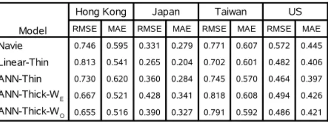
The inverse relationship between unemployment rate and inflation (Phillips curve) exists in all cases, and the his-torical inflation significantly affects the current inflation as well in all cases. It is not surprising that the global-ization factor is very significant in the linear model for each sample country, and it does generate the downward tendency in inflation through time with different levels. Table 1 presents all the summary forecast error statis-tics, root-mean-squared error (RMSE) and mean abso-lute error (MAE), for each sample country. As previ-ously discussed, in the first few out-of-sample test pe-riods, we might be able to decide which ANN performs best, but some ANNs still have similar performances after some test periods. If this situation happens, thick mod-els (ANN thick with equal weight and ANN thick with unequal weight models) can be accordingly applied. Ex-cept for the linear, ANN thin and thick models, a simple naive model producing the benchmark forecast is also in-cluded. Basically, there are five different forecasting mod-els, which are naive, linear, ANN thin, ANN thick with equal weight (ANN-Thick-WE), and ANN thick with

un-equal weight (ANN-Thick-WO) models.

Some significant observations emerge from our empirical results in Table 1. First, there are two (Hong Kong and

Table 1: Forecast Accuracy for Inflation of Sample Coun-tries

the US) out of four cases, in which either ANN thin or thick models outperforms the naive and best linear mod-els. This result is very encouraging because we do not make any claim on the optimality of the ANN models that are merely based upon these repeatedly-updated and well-specified linear models. As previously mentioned, al-though the ANNs have the same inputs as the best linear model, the variations on learning rates, number of neu-rons in each layer, and number of training cycles could generate a lot of different ANN models that might lead to different forecasting performances. Nevertheless, ob-taining optimal values for so many ANN models is rather time-consuming and complex. In the case of Hong Kong (and all other cases indeed), we use the average of all forecasts from the different ANNs in the first 10 out-of-sample test periods, because we could not determine which ANN is the best without any performance history. Afterward, we use the forecasting performances from the first 10 test periods to obtain the weights in order to com-bine weighted forecasts for the next test period, and we update the weights before each test period. Actually, the weights vary just a little each time as the new information rolls in. This indicates that weights could become stable after some test periods in the case of Hong Kong if we have more data available. However, due to the constraint of data availability, we do not expect to get the optimal weights within some test periods, which could be possibly improved by using longer test periods with more experi-ences. Hong Kong is the only case in which the ANN thick with unequal weight (ANN-Thick-WO) model

out-performs all other models in this study with substantially lower RMSE and MAE. In the case of the US, the ANN thin model outperforms all other models. Thirdly, in the cases of Taiwan, the ANN thin model performs as well as the best linear model, and it significantly outperforms the naive model. Fourthly, in the case of Japan, the linear model has the best forecasting performance, and neither the ANN thin nor the ANN thick model can outperform the naive model. Lastly, the ANN thick with unequal weight model in all cases do outperform the ANN thick with equal weight model despite the fact that they are not the best in some cases.

is very hard to obtain all the optimal parameters (e.g., learning rate, number of neurons in each layer, number of training cycles, etc.) for so many ANN candidate mod-els through a very time-consuming and complex process. The focus of this study was on a real time forecasting with many repeated estimations and sample countries, so se-lecting the variables for the ANN based upon the best linear model is only a compromise between practicality and optimality. However, our results are very encourag-ing.

4

Conclusions

In this paper, we study the globalization influences on forecasting inflation in an aggregate perspective using the Phillips curve for Hong Kong, Japan, Taiwan and the US by artificial neural network-based thin and thick mod-els. Our empirical results support that globalization in-fluences do generate the downward tendency in inflation through time in all cases. Either the ANN thin or the ANN thick model that has been developed upon the best linear model for each country in this study has shown significant superiority over the naive model in most cases and over the best linear model in some cases. In fact, finding optimal values for the large number of parameters involved in the ANN models is rather difficult, and thus we do not make any claim on the optimality of our ANN models. Even though our empirical results are not over-whelmingly satisfactory, building the ANN model based upon the best linear model is a good compromise between practicality and optimality, which sheds strong light for future work such as cross-validations and sensitivity anal-ysis for selecting variables to enhance the ANN’s perfor-mances. In addition, whether or not obtaining the op-timal parameter values (time-consuming and unpractical task) is essential to conspicuously enhance the ANN’s performances to a very satisfactory level could be an is-sue to study as well.

References

[1] I. M. Fund, “World economic outlook apirl 2006: Globalization and inflation,” April 2006.

[2] J. H. Stock and M. W. Watson, “Forecasting infla-tion,”Journal of Monetary Economics, vol. 44, no. 2, pp. 293–335, 1999.

[3] M. Hinich and D. Patterson, “Evidence of nonlinear-ity in daily stock returns,” Journal of Business and Economic Statistics, vol. 3, no. 1, pp. 69–77, 1985.

[4] N. Sarantis, “Nonlinearities, cyclical behaviour and predictability in stock markets: international evi-dence,” International Journal of Forecasting, vol. 17, no. 3, pp. 459–482, 2001.

[5] P. Ammermann and D. Patterson, “The cross-sectional and cross-temporal universality of

nonlin-ear serial dependencies: evidence from world stock indices and the Taiwan stock exchange,” Pacific-Basin Finance Journal, vol. 11, no. 2, pp. 175–195, 2003.

[6] P. McNelis and P. McAdam, Forecasting Inflation with Thick Models and Neural Networks. Working Paper Series 352, European Central Bank, 2004.

[7] T.-F. Hu, H. C. Su, and I. Gondra Luja, “Examining nonlinear interrelationships among foreign exchange markets in the pacific basin with artificial neural net-works,” inPDPTA’07- The 2007 International Con-ference on Parallel and Distributed Processing Tech-niques and Applications, pp. 829–835, June 2007.

[8] A. Atkeson and L. E. Ohanian, “Are phillips curves useful for forecasting inflation?,” Federal Reserve Bank of Minneapolis Quarterly Review, vol. 25, no. 1, pp. 2–11, 2001.

[9] C. W. J. Granger and Y. Jeon, “Thick modeling,” Economic Modeling, vol. 21, no. 2, pp. 323–343, 2004.

[10] T. Mitchell,Machine Learning. McGraw-Hill, New York, 1997.

[11] N. Gershenfeld and A. Weigend, Time Series Pre-diction: Forecasting the Future and Understanding the Past, pp. 1–70. Addison-Wesley, 1993.

[12] F. Rosenblatt, “The perceptron: A probabilistic model for information storage and organization in the brain,” Psychological Review, vol. 65, no. 6, pp. 386–408, 1958.

[13] A. Bryson and Y. Ho, Applied Optimal Control. Blaisdell, New York, 1969.

[14] D. Rumelhart, G. Hinton, and R. Williams, “Learn-ing representations by back-propagat“Learn-ing errors,” Na-ture, vol. 323, pp. 533–536, 1986.