in Brazil?
Tito Nícias Teixeira da Silva Filho
†
, Francisco Marcos Rodrigues
Figueiredo
‡
Contents: 1. Introduction; 2. Core Inflation: Where Do We Stand?; 3. Desirable Statistical Properties of a Good Core Inflation Measure; 4. Core Inflation in Brazil; 5. Improving Core Inflation Measurement in Brazil; 6. Empirical Results; 7. Conclusion; A. Appendix.
Keywords: Core Inflation, Inflation, Supply Shocks, Relative Prices, Volatility. JEL Code: C43, E31, E52.
This paper assesses the performance of the core inflation measures calculated by the Brazilian Central Bank (BCB). The evidence shows that they do not meet some key statistical criteria that a good core inflation measure should have: unbiasedness and the ability to forecast infla-tion. That performance stems, in part, from the lack of a well-grounded statistical and economical basis underlying them. Three new measu-res are built and assessed using the same criteria. The evidence shows that although their behaviour is more in accordance to what the theory claims, they still lack the ability to help forecasting inflation. Hence both the BCB and the market should use core inflation cautiously.
Este artigo avalia o desempenho das medidas de núcleo de inflação cal-culadas pelo Banco Central do Brasil (BCB). A evidência mostra que elas não satisfazem alguns critérios-chave estatísticos que uma boa medida de nú-cleo deve ter: ausência de viés e capacidade de prever a inflação. Esse resul-tado advém, em grande parte, da falta de uma base estatística e econômica sólida dos núcleos. Três novas medidas são construídas e avaliadas. A ev-idência mostra que, apesar de o seu comportamento estar mais de acordo com o que a teoria prediz, elas ainda não ajudam a prever a inflação. Por-tanto, tanto o BCB como o mercado devem utilizar o núcleo de inflação com cuidado.
∗The authors would like to thank Patrice Robitaille, Fernando de Holanda Barbosa, Fabio Araujo and Nelson Sobrinho for
valu-able comments and suggestions as well as seminar participants at the XIV Meeting of the Central Bank Researchers Network (CEMLA) and at the Central Bank of Brazil. We are also thankful to Alfredo de Oliveira for kind assistance with the data. The views expressed in the paper are those of the authors and do not necessarily reflect those of the Central Bank of Brazil.
†Central Bank of Brazil. E-mail:[email protected]
1. INTRODUCTION
“After a jittery few weeks, bond markets rallied on June 15th on news that America’s core consumer price index rose by just 0.1% in May. (. . . ) What markets blithely ignored was the day’s bad news. Headline consumer prices rose by 0.7%, the biggest monthly increase for nearly two years. (. . . ) For bond prices to rise on such a big jump in inflation, markets must be placing a great deal of faith in the core index as the true gauge”.
(The Economist, June 2007)
Boosted by the adoption of inflation targeting (IT) frameworks by several central banks since the end of the 1980s, core inflation has increasingly become popular among policymakers and market partici-pants. That popularity has not been, however, endorsed by their actual performance. Dismal evidence on their accomplishments, questions about their real capabilities as well as criticism on the weight some central banks give to them have been growing. This should not come as a surprise given, for example, the well-known difficulties in separating inflation noise from signal.
Curiously, however, since core inflation measures have begun to be calculated in Brazil, in 2000, following the adoption of the IT regime, they have remained unquestioned. This is surprising not only because of the dissent mentioned above but also because of how they have fared so far. Moreover, the Brazilian economy has historically been subject to frequent economic shocks. In reality, not only core inflation is closely watched by market participants in Brazil – as elsewhere – but there has been a widespread emergence of “alternative” core inflation measures, such as core measures for tradables, non tradables and service goods, among others (e.g. A. C. Pastore e Associados, 2008).1 An exception
to that complacency is the paper of da Silva Filho (2008), who shows disturbing evidence regarding the performance of the so-called exclusion core in Brazil.
This paper not only is the first one to assess the three core inflation measures that have been calculated by the Central Bank of Brazil since 2000, but also aims to look at core inflation on a broader perspective.2 Firstly, it assesses whether those measures are doing a good job (i.e. are they delivering
what one expects from a good core inflation measure in terms of its statistical properties?). Secondly, it proposes new – theoretically sounder – measures of core inflation for Brazil. Finally, although country specific, the overall results are assessed taking into account evidence for other countries, aiming at building a broader picture about the real capabilities of core inflation.
The evidence shows that core inflation measures have not been doing a good job in Brazil. Their bias is either statistically significant or economically relevant. Moreover, they have poor dynamics and do not seem helpful in explaining near term inflation. Three new core measures are built and assessed: two exclusion cores and a double weighted core. The results show that they have better statistical properties, especially regarding the bias criterion. Nevertheless, despite the improvements they remain adding little information, beyond that already contained in the history of headline inflation, to explain near term inflation.
The structure of the paper is as follows: Section 2 gives a glimpse on the core inflation debate. Section 3 presents what the literature considers to be the most desirable properties of a good core inflation measure. Section 4 introduces the core measures calculated by the Central Bank of Brazil (BCB), and assesses their performance since 1996, with special emphasis on the IT period. Section 5 introduces three new measures of core inflation for Brazil. Section 6 evaluates those measures and Section 7 concludes the paper.
1For example, Schwartsman (2008), a former BCB’s Deputy Governor, argued emphatically that the acceleration of inflation at
the time had a permanent nature since core inflation was also rising.
2Notice that, as of January 2010, influenced by a preliminary version of this work, the Central Bank of Brazil has decided to stop
2. CORE INFLATION: WHERE DO WE STAND?
Core inflation measures are around us since the 1970s, and ever since both the public and economists have generally taken them for granted. However, despite their popularity and widespread use by many policymakers, core inflation remains a controversial matter. The dissent, which has been growing in recent years, can be viewed on several dimensions. On theoretical grounds, economists could not even agree on what core inflation means. The most popular definition associates core inflation to underly-ing inflation, or, in other words, to what remains after the “noise” is taken out of the inflation rate. Noise stands for temporary price developments. As Blinder (1997) puts “The name of the game then was distinguishing the signal from the noise, which was often difficult.” Perhaps, more intuitively, core inflation could be seen as a measure that uncovers the “true” underlying trend of inflation (Bryan et al., 1997). The trend would represent the most persistent, enduring or durable part of inflation.
Core inflation has also been defined in a related but different viewpoint, based on its forecasting ability. In that case it is considered to be that part of inflation that is most helpful to predict headline inflation. Blinder (1997) argues that: “To me, the durable part of the information in each monthly inflation report was the part that was useful in medium – and near-term inflation forecasting.” It has been defined (or expressed) in other ways as well, such as that part of inflation which is most correlated to money growth (Bryan and Cecchetti, 1994), the part which is not correlated to medium-long run real output (Quah and Vahey, 1995), or that component of inflation common to a large number of individual price series (Bryan and Cecchetti, 1993), among others.
Nonetheless, an intuitive and simple way of formally defining core inflation is to assume that changes in the price of an individual good or service can be divided into two parts: a common compo-nenteπt, represented by the trend, and an idiosyncratic partεi,t, represented by (transitory) deviations around that trend.
πi,t=eπt+εi,t (1)
Hence (1) defines the rate of change of the price of an individual goodi,πi,t = ∆ lnPi,tas con-sisting of an aggregate inflation component, eπt = ∆ lnPet, and a relative price change component
εi,t, which acts just as noise. The problem of measuring core inflation is precisely how to isolate these two components from observed price changes. Thus, core inflation (πtc) could simply be defined by this common component:
πtc=eπt (2)
Several methods aimed at measuringπc
t can be found in the literature. Most of them are basically strategies for excluding or down weighting items from the price indices based on some criterion, usu-ally volatility. To a summary of alternative ways to build core inflation measures see Silver (2007) and Wynne (1999).
On practical grounds, despite its increasing use by central banks in recent years – which has been boosted by the adoption of inflation targeting (IT) regimes in several countries – there has been some disenchantment with core inflation. From a policymaker’s perspective, for example, some central banks that used to establish their inflation targets in terms of core inflation (Australia, New Zealand and Czech Republic), have changed their minds and now aim at keeping inflation in line with targets set for headline inflation. In other cases, the targeted indexes, which excluded interest rates effects, have been ruled out in favour of headline inflation (e.g. South Africa and the UK).3Moreover, in some countries,
such as Canada, where core inflation is used as anoperationalguide, the “official” core has been replaced by a supposedly better one, showing the dangers of relying too much on any specific core measure.
3Since the rationale for excluding interest rate effects is different from that for excluding volatile items, those indexes can hardly
Indeed, if there is a consensus about core inflation today it is that no specific measure dominates others in all dimensions and criteria [see Hogan et al. (2001) for Canada, Mankikar and Paisley (2002) for the U.K, and Rich and Steindel (2007) for the U.S.].
Core inflation also seems to have lost terrain among economists. For instance, after being one of its main enthusiasts [e.g. Bryan and Cecchetti (1994) and Cecchetti (1997)], Cecchetti (2006) has become disappointed with their actual performance. He notes that “The techniques [for construction of core measures] rely on various statistical methods, but in the end all we are doing is forecasting – and not terribly good forecasting at that.” He concludes that policymakers “. . . should turn their attention to forecasts of headline inflation and stop focusing on core measures.” Bean (2006) calls to attention the theoretical inconsistency of traditional exclusion core measures (i.e. that excludes food and energy). He argues that “. . . to me renders suspect the practice of focusing on measures of core inflation that strip out energy prices, while retaining the falling goods prices.” King (2007) agrees and warns that “. . . measures of ‘core inflation’ that strip out certain prices can be highly misleading.” Nonetheless, the so-called exclusion core is precisely the most popular one, especially in the U.S.
Marques et al. (2003) and Clinton (2006) follow a different road and question the supposedly the-oretical predictive content of core inflation. They argue that it is not suitable for forecasting headline inflation in the near term, since the latter is heavily influenced by transitory factors, which is exactly that part of inflation that core inflation tries to ignore.4 On the other hand there are also core inflation
enthusiasts, such as Blinder (2006), who argues emphatically about the central role that core inflation should play in monetary policy-making. According to him one main reason why central banks should follow closely (traditional) core inflation is not because it is less volatile than headline inflation but rather because “. . . monetary policy is unlikely to have much leverage over energy (or food) prices; so it makes sense to focus the central bank’s attention on the inflation it can actually do something about.” Moreover, according to him a key property of core inflation is exactly its forecasting ability. Finally, there are also those, such as Mishkin (2007), who recognise the poor performance of traditional core measures but nonetheless still think they have an important role to play in monetary policy. For ex-ample, he argues that by focusing on core inflation policy responses will produce less volatility in both output and inflation.
Central banks, in their turn, have been criticised for putting too much emphasis on core inflation when setting monetary policy. For example, Laidler and Aba (2000) criticised the supposedly complacent reaction of the Central Bank of Canada in face of rising headline inflation, since core inflation continued to be well behaved. Using the same reasoning The The Economist (2007) criticised both the Fed and the market for putting too much emphasis on core inflation while headline inflation was rising.
The suspicion about core inflation seems to lie essentially on its actual performance rather than in its theoretical underpinnings, even though, as seen above, the latter is not uncontroversial. More-over, although most criticism refers to the traditional core measure, it also encompasses other types of cores. For instance, the OECD (2005) analysed the performance of a variety of core measures in sev-eral countries and, in many cases, they bear problematic features. In various cases headline inflation was not attracted to core inflation, what, in theory, should happen with good cores. Evidence of bias, among other problems, was also widespread. Smith (2004) also found evidence of bias among several core measures for the U.S., Rich and Steindel (2005) found evidence that “. . . no core measure does an outstanding job forecasting CPI inflation.”, while Bryan and Cecchetti (1994) found evidence for the U.S. that headline inflation is a better predictor of itself than the traditional ex-food & energy core. Some disturbing evidence comes from Gavin and Mandal (2002), whose findings suggest that food prices do contain useful information about trend inflation in the U.S. Moreover, they find that food prices are a better inflation predictor (for inflation in the next two years) than the traditional core inflation, which exclude them.
4Clinton also argues that core inflation is not a good predictor of headline inflation in Canada, and that the inflation target itself
Given the above dissent it should not come as a surprise that different central banks face and use core inflation in different ways. While the Fed puts great emphasis on core inflation when moving interest rates, both the Bank of England and the ECB focus mainly on headline inflation, while the Bank of Canada uses it as an operational guide. In Brazil, although the emphasis is on headline inflation, the Central Bank calculates three different measures of core inflation, which are used – along with many other indicators – to help assessing current and future inflation developments.
Notwithstanding the different emphasis given by central banks and the dispute around it, there is no doubt that core inflation plays an important role – sometimes central – in modern monetary policy. Therefore, it is imperative for policymakers to be aware of and to have an accurate view about the real capabilities of core inflation measures; that is, their virtues and limitations.
3. DESIRABLE STATISTICAL PROPERTIES OF A GOOD CORE INFLATION MEASURE
Regardless of whether the dissent about core inflation is theoretically or empirically based, it is largely agreed that an ideal core inflation measure should possess at least some desirable statistical features. First, it seems obvious to argue that a good core inflation measure should not be biased. Bias is usually assessed in two ways. In the first, the means of headline and core inflation are calculated for a given period and the results are compared in order to check if they diverge in a statistically significant way. The hypotheses can be stated as:5
H0 : T−
1
T X
1
πct =T−
1
T X
1
πt (3)
H1 : T−
1
T X
1
πct 6=T−
1
T X
1
πt (4)
whereπt = ∆pt = ∆ lnPtandπtc = ∆pct = ∆ lnPtc stand for headline and core inflation, respec-tively, andPt andPtcare the headline and core price levels.
Another possibility is estimating the following equation
πt=α+βπtc+εt (5)
and test the null joint hypothesis thatα= 0andβ = 1. If the null is accepted it means that the core under analysis is not biased.
Second, a good measure of core inflation should be able to capture/track ascloselyas possibletrend
inflation.6 Two questions arise here. First, how is trend inflation determined? Second, what do we mean by “ascloselyas possible”? As to the first question, economists have devised several methods and identification assumptions to extract a trend from a given time series. A very popular method is the Hodrick-Prescott (HP) filter. Another one is the unobserved components (UC) model, which uses the Kalman Filter (KF). In the core inflation literature, however, the most used method is simply the centred moving average (CMA) of headline inflation, a procedure advocated by Bryan and Cecchetti (1994). In this case, how many periods should one use? In other words, how smooth or persistent should the trend be?
5It should be called to attention that this test is sometimes carried out using the ANOVAF-statistic (e.g. Catte and Sløk, 2005).
However, since the two variables are likely to have different variances (indeed, a major objective of core inflation measures is lower variance compared to headline inflation) this testing procedure is inappropriate.
6Note that the criterion is tightly linked to the first one, since the ability to track trend inflation depends on whether or not core
The higher the number of periods used in the calculations the smoother/more persistent will the trend be and the smaller the influence of the most recent observations. This remark brings out two issues. First, there is no such a thing like “the” trend: trends differ according both to the period they refer to and to the method chosen. There are shorter, medium and longer term trends, and they could coexist while being different. If inflation is stable they tend to coincide. Second, which horizon should the central bank care the most? One could argue that by focusing on the long-term inflation trend the central bank could end up accommodating persistent deviations of headline inflation from the target (trend). On the other hand, by putting too much emphasis on a volatile trend – a feature usually asso-ciated with shorter-term trends – the central bank could increase both output and inflation volatility unnecessarily. Since the central bank main interest lies on inflation developments over the near future, that is, over the horizon it can actually act upon, the shorter to medium term inflation trend seems to be the most relevant for monetary policy.
As to the second question, two criteria are usually used to gauge how close core inflation is from trend inflation. The first is the root mean square error (RMSE) (equation 6), and the second is the mean absolute deviation (MAD) (equation 7). The core measure that minimizes the chosen criterion would, in principle, be the best one.
RM SE=T−1/2
v u u tXT
t=1 πc
t−πttrend 2
(6)
M AD=T−1
T X
t=1
πtc−πttrend
(7)
Finally, and most importantly, it is largely agreed (although there is no consensus) that core inflation will be most useful to monetary policy if it helps to predict headline inflation.7More precisely, given the
information set available to a forecaster, one would like to know if the additional information provided by core inflation helps to predict inflation. However, given that this information set is a potentially very large one, the assessment will be done within a narrower scope. It seems obvious to argue that, among the myriad of variables that are part of the information set used by a forecaster, the history of inflation is certainly present. Therefore, the test used here aims at checking if, conditional on past headline inflation rates, core inflation brings any useful information to explain future headline inflation.8 Given
the well documented fact that simple univariate inflation forecasting models are a tough benchmark to beat [see, for example, Canova (2002)], this should not be a serious shortcoming when doing inference. Indeed, if core inflation is not informative when one controls for inflation lags, it is unlikely to be helpful once other variables are added to the forecasting model.
Hence, one way to assess this requirement is to use a specification like (8). Three forecast horizons will be focused here: 2, 3 and 4 quarters.9
∆kpt+k=µ+
I X
i=0
αi∆pt−i+
J X
j=0
βj∆pct−j+εt+k (8)
where∆kpt= lnPt−lnPt−k is inflation overkquarters,Ptis the quarterly IPCA (Broad Consumer
Price Index) price index and∆ptand∆pctare, respectively, quarterly headline and core inflation. Hence,
7Ideally, core inflation should also act as a predictor of inflation turning points, a valuable information for any policymaker.
8This test is known in the literature as the Granger-“causality” test.
9Estimates for Brazil suggest that changes in the interest rate begin to act upon the inflation rate in a statistically significant
equation (8) provides multi-step forecasts for inflation over several horizons, using quarterly data.10
One consequence of such a set up is that forecasting errors will have moving average dynamics, since forecast periods overlap. This feature makes inference unreliable, and potentially wrong, since, for example, traditional standard errors statistics are invalid.
One way to avoid this problem is to change the frequency of the data to match the forecasting horizon desired, according to equation (9).11
∆kpt+k =µ+
12/k X
i=0
αi∆kpt−ki+
12/k X
j=0
βj∆kpct−kj+εt+k (9)
The literature also lists other features/criteria as being important, but we believe the above ones are the most relevant. Moreover, some of them do not have our sympathy. For instance, it is argued that a good core inflation measure should be simple and easily understandable by the “public” (e.g. Rich and Steindel, 2005). This argument seems highly overstated. How understandable the concepts of, say, asymmetric trimmed mean or dynamic factor models are for a layman? Actually, the “public” often has difficulty in understanding some simple economic concepts such as the very concept of inflation. Moreover, many issues central to monetary policy-making are complex even to economists, let alone the “public”.
It is also argued that core inflation should be less volatile than headline inflation. We do not have any quarrel with that, but we feel this requirement has been overly emphasized. Indeed, for the vast majority of available methods core inflation will be less volatile than inflationby construction. Finally, some of the tests found in the literature do not really tackle the issue under analysis. For example, the following “naïve” model is used to check whether recent changes in core inflation are informative about future changes in headline inflation (see Catte and Sløk, 2005).
∆12pt+12−∆12pt=α+β ∆kpct−∆kpct−k
+εt+j (10)
where, for example,k= 3,6,9and12when monthly data is used.
A major problem here is that (10) is very likely to be mis-specified, preventing any reliable inference. For example, it does not even include lags of headline or core inflation. Hence it is not surprising that for most of the cases and countries Catte and Sløk (2005) found theβ coefficient to be insignificant. The lack of significance does not say much, since changes in core inflation could actually be helpful in predicting inflation once other relevant variables are added to the model. Indeed, in the few cases where the regressor was significant, its sign was theoretically wrong, a typical symptom of the omitted variable problem.
4. CORE INFLATION IN BRAZIL
The Central Bank of Brazil (BCB) currently calculates three core inflation measures.12 The first one is a traditional exclusion core in which food (at home), energy and regulated & administered prices are excluded. Regulated prices are those prices that follow specific rules laid out in contracts. They refer to utilities, such as electricity and telephony, which have been privatised as of 1995. In its turn, administered prices are those prices that although not being set by contracts are determined by the Government (whether federal, state or municipal). Remedy, fuel prices (with the exception of ethanol) and municipal taxes are some examples.
10Note that regardless of the frequency of the data used in the models, the core inflation measures used in this paper are
constructed using monthly data, which are then aggregated to lower frequency data.
11Nowkindicates both the frequency of the data and of the forecast.
The second measure is a (symmetrical) trimmed mean core, where 20% of prices changes are ex-cluded from both tails of the monthly price distribution. The third core is a smoothed (symmetrical) trimmed mean core, where mainly regulated & administered prices changes are “smoothed” before the trim.13 Since those prices are changed infrequently, when the change occurs it is usually (relatively)
large and, therefore, likely to be trimmed. However, after being smoothed (i.e. the change is divided equally in the current and next eleven months) the trim becomes much less likely.14
The calculation of core inflation measures in Brazil started after the implementation of the inflation targeting (IT) framework in mid-1999.15 This was not a coincidence; on the contrary, core measures were devised to help monetary policy decisions within the new monetary policy framework. The first time the concept of core inflation was officially mentioned by the BCB was in the notes of the 45th Copom’s (monetary policy committee) meeting, which took place in March 2000, when it referred to a CPI core measure calculated by the Getulio Vargas Foundation.16,17The first time the BCB referred to a
core inflation measure of its own was in the notes of the 50th Copom’s meeting (August 2000), when it referred to the smoothed trimmed mean core. One year later, in the notes of the 63th Copom’s meeting (September 2001), the BCB introduced the exclusion core. Finally, the BCB mentioned for the first time the trimmed mean core in the June 2003 Inflation Report.
This section assesses how those three core inflation measures have fared so far according to the criteria laid out above. Their performances will be assessed for the post-stabilization period, since high inflation heavily distorts relative prices and could affect the results in an idiosyncratic way. More precisely, the sample refers to the 1996–2008 period.18Within that period, we are particularly interested
in their performances during the inflation targeting period (i.e. 1999–2008).
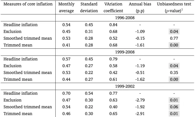
Table 1 shows the unbiasedness test results (together with some descriptive statistics). The results are far from encouraging. For example, two out of the three core inflation measures – the exclusion and the trimmed mean cores – show bias for both the whole sample and the inflation targeting period.19 Not only those biases are statistically significant but their sizes areeconomicallyrelevant. While the exclusion core bears a bias of 1.2 p.p. during the IT period, the trimmed mean’s bias reaches 1.6 p.p. In addition, although not statistically significant, the smoothed trimmed mean core delivers a bias of half of a percentage point during the IT period, a magnitude that is economically relevant (i.e. it suffices to both interfere in agents’ planning and central bank’s monetary policy).20 Finally, the results from Table
1 show that, on average, all core inflation measures have underestimated IPCA inflation for more than one decade. The underestimation was particularly severe in the first years of the floating/IT regime (1999–2002) – precisely when they were most needed – when the bias reached almost three percentage
13Tobacco and tuition are smoothed although their prices are not regulated or administered. For further details on the
method-ology see Figueiredo (2001).
14For conciseness, throughout the rest of the paper the denomination “trimmed mean core” will be used to refer to the
non-smoothed (symmetrical) version of the trimmed mean core.
15The inflation targeting framework was officially adopted in Brazil through the Decree No 3088 of June 21st 1999.
16To a summary of the first steps on core inflation measurement in Brazil outside the BCB see BCB (2000) and Figueiredo (2001).
17In the notes of the 46th and 47th Copom’s meetings the BCB also mentioned the concept of core inflation, even though it those
cases it did not stated to what specific measure it was referring to.
18The Real Plan was implemented in July 1994. The exclusion and trimmed mean cores’ historical series go back until January
1995; however, the data for the smoothed trimmed mean core is available from January 1996 onwards only.
19Of course, since both periods overlap a great deal one expects results to be similar.
20At this point the following remark by Blinder (1997) is useful: “For I can tell you from personal experience that a full percentage
Table 1: Descriptive statistics for IPCA core inflation measures*
Measures of core inflation Monthly Standard VAriation Annual bias Unbiasedness test average deviation coefficient (p.p) (p-value)1
1996-2008
Headline inflation 0.54 0.45 0.84 -
-Exclusion 0.45 0.31 0.68 -1.09 0.04
Smoothed trimmed mean 0.53 0.28 0.52 -0.15 0.77
Trimmed mean 0.41 0.28 0.68 -1.61 0.00
1999-2008
Headline inflation 0.57 0.45 0.79 -
-Exclusion 0.47 0.27 0.58 -1.19 0.04
Smoothed trimmed mean 0.53 0.22 0.42 -0.51 0.35
Trimmed mean 0.44 0.27 0.61 -1.62 0.00
1999-2002
Headline inflation 0.70 0.54 0.77 -
-Exclusion 0.47 0.30 0.63 -2.79 0.01
Smoothed trimmed mean 0.54 0.22 0.40 -1.92 0.06
Trimmed mean 0.46 0.30 0.65 -2.91 0.01
(*) Shaded areas highlight statistical significant tests at 6%.
(1) This is the mean equality (unbiasedness)t-test which allows for unequal variances.
points for the exclusion and trimmed mean cores.21 Moreover, even the smoothed trimmed core, which
is unbiased when the longer sample is considered, was seriously biased in that four-year period. At this point a warning is required. Focusing only on the existence of bias over an extended period of time – a pervasive feature in the literature – could be misleading, and generally leads one to miss the point.22 As Figure 1 shows, although the smoothed trimmed mean core has a small (statistically
speaking) bias when a longer sample is considered, its dynamics is troublesome. More specifically, it is piecewise biased over long enough periods of time – a feature quite relevant for monetary policy – but in opposite directions such that they offset each other in longer samples.
Note that the smoothed trimmed mean core sizably underestimated headline inflation during the four years following the floating (1999–2002), and overestimated it in the next four years (2003–2006). That could, for example, lead to a too lenient monetary policy in the first period and an unnecessarily tight monetary policy in the second one, should the central bank put too much emphasis on core inflation. Moreover, if economic agents also put a great deal of emphasis on core inflation when forming inflation expectations, those will be biased too.23 Finally, and most importantly, the evidence shows
21For a more detailed explanation regarding the behaviour of the exclusion core after the floating see da Silva Filho (2008), Section
4.
22Rich and Steindel (2007), for example, argue that “A core inflation measure should have a comparable mean to the goal inflation
series over a long period of time.”
23See da Silva Filho (2008) for evidence on the pattern of inflation forecasting errors in Brazil after the implementation of the IT
Figure 1: Smoothed trimmed mean core’ annual bias
(4p,p,) (3p,p,) (2p,p,) (1p,p,) 0p,p, 1p,p, 2p,p, 3p,p, 4p,p,
1996 1997 1998 1999 2000 2001 2002 2003 2004 2005 2006 2007 2008
that core inflation measures have not been successful in purging only transitory shocks from headline inflation.24
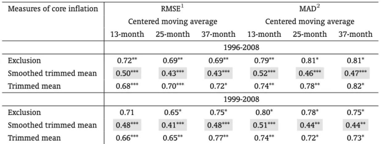
Table 2 shows how closely each core inflation measure tracks trend headline inflation (assuming it is well represented by a centred moving average). As can be seen, there is an overwhelming dominance of the smoothed trimmed mean core under this criterion. It easily beats the exclusion and trimmed mean cores – which have similar performances – in both samples, criteria and regardless of the number of months used in the moving average. Its relative volatility is less than half of headline inflation’s.25
Table 3 uncovers interesting evidence on the usefulness of core inflation in explaining headline inflation over the near future in Brazil. The first line shows the estimation results of a restricted version of equation (7) – one in which only lags of headline inflation enter (i.e. the betas are set to zero). The other lines show the results when each core inflation measure is added to the restricted specification separately. Two results stand out: first, the extremely lowR2
statistic, which shows that headline and core inflation over the previous four quarters are not very informative about inflation over the next 2, 3 and 4 quarters, during the sample analyzed, for Brazil. More strikingly, when core inflation is added to the model the equation’s standard error actually increases, with the exception of the trimmed mean core in the 2 and 3-quarter ahead cases.
Second, Table 3 also displaysF-test statistics – whose null is that all the coefficients attached to lags of core inflation are zero – and the results are intriguing. When traditionalF-tests are (incorrectly) used they easily accept the null in all cases. Nevertheless, when Andrews (1991) heteroscedasticity and autocorrelation consistent standard errors (HACSE) are used the null is rejected in all cases. Although the presence of autocorrelation can sharply distort standard test statistics, it is eye-catching the
sub-24Indeed, as Figure 5 shows, during the 1996–2003 period the bias of the exclusion and trimmed mean cores is quite large (
−1.9
p.p. and−2.3 p.p., respectively). In the most recent period (2004–2008) the former turns out not to be biased. And, although
the bias of the latter is smaller (−0.8 p.p.), it continues to be quite relevant.
25Rigorously, the term relative volatility applies when both headline and core inflation share the same trend. Since we have
Table 2: Deviations from trend IPCA inflation
Measures of core inflation RMSE1 MAD2
Centered moving average Centered moving average 13-month 25-month 37-month 13-month 25-month 37-month
1996-2008
Exclusion 0.72** 0.69** 0.69** 0.79** 0.81* 0.81*
Smoothed trimmed mean 0.50*** 0.43*** 0.43*** 0.52*** 0.46*** 0.47***
Trimmed mean 0.68*** 0.70*** 0.72* 0.74** 0.78** 0.82*
1999-2008
Exclusion 0.71 0.65* 0.75* 0.80* 0.78* 0.75*
Smoothed trimmed mean 0.48*** 0.41*** 0.48*** 0.51*** 0.44** 0.44**
Trimmed mean 0.66*** 0.65** 0.77** 0.74** 0.72* 0.73*
*, ** and *** indicate significance at 10%, 5% and 1%, respectively, in Diebold & Mariano’s test for predictive accuracy.
The test aims to test the null hypothesis of equality of expected forecast accuracy against the alternative of different
forecasting ability across models, where forecast accuracy is measured according to a chosen loss function.
(1) Root mean square error relative to that of headline inflation.
(2) Mean absolute deviation relative to that of headline inflation.
Table 3: Goodness of fit andF-tests results
2Q ahead 3Q ahead 4Q ahead
R2 σˆ F
1 F2 R2 ˆσ F1 F2 R2 σˆ F1 F2
Headline 0.08 1.22 - - 0.07 1.43 - - 0.09 1.71 -
-inflation
Exclusion 0.11 1.23 0.52 0.00/0.21 0.10 1.47 0.71 0.02/0.45 0.12 1.78 0.94 0.07/0.66
Smoothed 0.11 1.25 0.62 0.00/0.10 0.09 1.46 0.44 0.00/0.12 0.11 1.74 0.39 0.00/0.25
trimmed mean
Trimmed mean 0.13 1.16 0.11 0.00/0.09 0.10 1.40 0.23 0.00/0.02 0.12 1.74 0.60 0.00/0.20
(1) Tests are based on equation (5) augmented by intervention variables. The following dummies were required for model congruence (apart from
autocorrelation), in the 2, 3 and 4-quarter ahead cases, respectively: 2002.4 and 2003.1, the latter plus 2003.2 and the latter plus 2003.3.F1shows
thep-value of the traditionalF-test, where the null is that all core inflation lags have zero coefficients.F2refers to thep-value when theF-test
uses heteroscedasticity and autocorrelation consistent standard errors (HACSE). The firstp-value comes from theF-statistic that uses errors based
on the procedure of Andrews (1991), while the second is based on the procedure of Newey-West (1987). In order to highlight the low explanatory
power of both headline and core inflation over future inflation, theR2statistic comes from equation (5), since the inclusion of dummies produces
a sharp increase in that statistic and could induce one to think that headline and core inflation (over the last four quarters) explain a sizable part of
future inflation. Sigma stands for the equation’s standard error. Shaded areas indicate the cases when the two correctedF-statistics reject the null
stantial changes in theF-statistic in the 2-quarter ahead case, when the degree of autocorrelation is lower (in the sense that the overlap is of just one period).26 At this point it is important to say that,
apart from autocorrelation, all models passed easily in all diagnostic tests.27’28 Hence, when standard
errors are corrected using the Andrews procedure,F-tests suggest that all three core inflation measures are helpful in explaining inflation in the near future.
However, when standard errors are corrected using the Newey-West procedure, the qualitative re-sults revert once again. Indeed, with the exception of the trimmed mean core for the 3-quarter ahead horizon – when the Andrews and Newey-West basedF-tests concur at 5% significance level but con-flict with the traditionalF-test – the Newey-West basedF-tests and traditionalF-tests are always in agreement. In other words: not only did the Newey-West correction end up not making any difference (compared to the traditionalF-test) in terms of qualitative inference, but its results conflicted with the
F-test based on the Andrews procedure.29 This fact is unsettling.
Despite the relevance of this conflicting evidence on the current investigation it requires a research of its own, which is not the aim here. It also calls for caution when inference is made using corrected standard errors, whose properties are usually well-established asymptotically only.30 Even so, Table
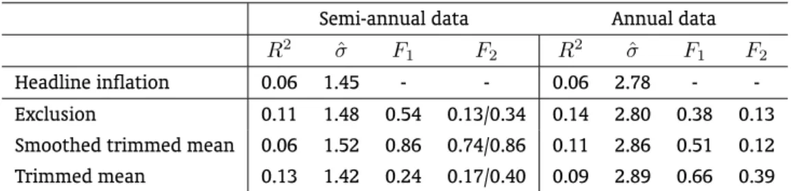
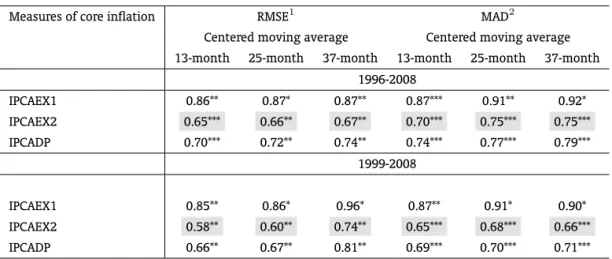
4 tries to uncover which evidence appears to be more reliable by displaying estimation results when lower frequency data is used, in order to avoid overlapping observations [i.e. equation (8)] Two horizons are focused: six-month ahead (i.e. semi-annual data) and one year ahead (i.e. annual data). The results suggest that the Newey-West correction has apparently been more successful in dealing with the effects of overlapping observations on test statistics than Andrews’, since the null is accepted in all cases. Hence, the evidence seems to imply that the three core inflation measures are not very informative in explaining inflation developments up to one year ahead.
Table 4: Goodness of fit andF-tests results (non overlapping observations)1
Semi-annual data Annual data
R2 ˆσ F
1 F2 R2 σˆ F1 F2
Headline inflation 0.06 1.45 - - 0.06 2.78 -
-Exclusion 0.11 1.48 0.54 0.13/0.34 0.14 2.80 0.38 0.13
Smoothed trimmed mean 0.06 1.52 0.86 0.74/0.86 0.11 2.86 0.51 0.12
Trimmed mean 0.13 1.42 0.24 0.17/0.40 0.09 2.89 0.66 0.39
(1) Tests are based on equation (5) augmented by intervention variables. A dummy for the second half of 2002 was required for
model congruence in models with semi-annual data. No dummy was needed for annual frequency models.F-tests are explained
in Table 3, where comments are also made for theR2statistic and sigma – the equation’s standard error. Note that since annual
models use only one lag, both the Andrews and Newey West procedure give the same value of theF-test statistic. Estimation
sample is 1997.1 – 2008.2 when semi-annual data is used and 1997 – 2008 when annual data is utilized.
Although Table 4’s estimation results come from models without overlapping observations – that passed in all diagnostics tests – it is interesting to check how the Andrews and Newey-West basedF
-26As expected, the p-value for the fourth order autocorrelation test decreases the longer the forecasting horizon is, since the
overlap increases.
27The following diagnostic tests were carried out in all estimations: Autocorrelation, ARCH, Normality, Hetero test, hetero-X test
and RESET test. For details see Hendry and Doornik (2001).
28It should be stressed that although the corrected standard errors also deal with heterocedasticity there were no signs of it in
all models (the p-value in all models are always greater than 0.5, and usually above 0.7).
29TheF-test based on Andrews correction is from the PcGive software while theF-test based on Newey-West correction is from
EViews.
statistics behave in this case. One would expect that in the absence of those problems they would be very similar to standardF-tests. However, even though the qualitative evidence remained the same at traditional significance levels, as expected, it is interesting to notice the large changes that can occur between the test statistics when there is no signs of autocorrelation and heterocedasticity. For example, thep-value for the exclusion core in the semi-annual data case reduces from 0.54 to 0.13, while the p-value for the trimmed mean core reduces from 0.51 to 0.12 in the annual data case. This evidence calls, once again, for caution when calculating tests statistics that use corrected standard errors. Finally, it is important to notice that when annual data is used in all cases lagged annual headline and core inflation were not statistically significant. This evidence concurs with theF-test results from quarterly models, whose lags encompass four quarters.
5. IMPROVING CORE INFLATION MEASUREMENT IN BRAZIL
The evidence laid out in the last section showed that both the exclusion and trimmed mean cores have not been doing a good job since they are biased and do not seem helpful in predicting headline inflation. As to the smoothed trimmed mean core, although its tracking ability is better it is piecewise biased during relevant periods of time, as Figure 1 shows. Moreover, it also does not seem helpful in predicting headline inflation.
The main (statistical) reasoning for excluding food and energy from headline inflation is that they are presumed to be highly volatile. There is also an implicitly and crucial (economic) reasoning, accord-ing to which those prices are mainly driven by temporary supply shocks. Figure 2 shows the volatility, measured by the standard deviation, of the nineteen sub-groups that are part of the IPCA, and scru-tinizes – for the three sub-periods defined below – if the volatility argument is corroborated by the data.31
The first sub-period goes from January 1995 until December 1998. This is basically the period after the implementation of the Real Plan, during which there was a fixed exchange rate (crawling peg) regime. The second sub-period goes from January 1999, when the exchange rate has begun to float, until December 2002, just before the beginning of the first mandate of President Lula da Silva. This period was marked by sharp exchange rate depreciation. The last sub-period begins in January 2003 and goes until December 2007, during which economic stabilization was consolidated and the exchange rate appreciated considerably.
As can be seen, the food at home sub-group is placed at the eighth place on the grid during the first period (1995–1998). Moreover, its volatility is pretty similar, for example, to transportation, clothing and health services sub-groups. During the second period (1999–2002), it was indeed among the most volatile sub-groups, and held the third place. However, during the last period (2003–2008) it went back to the sixth place. Therefore, contrary to common intuition, food – at least in its most aggregate level – is not among the most volatile sub-groups of the IPCA.32Thus, based on the volatility argument, one
sees that the food at home sub-group should not had been excluded from the headline index.
As to the energy “goods” notice that they are located in two sub-groups: in the “fuels and energy” sub-group – formed exclusively by energy items (household fuel and electricity) – and in the “motor fuel” item, within the transportation sub-group, which also comprises the “public transportation” and vehicles items.33 In this case the evidence is more supportive. The “fuels and energy” sub-group is
placed either in second or third place during the sub-periods above. However, at this level of
disag-31The IPCA components are defined, respectively, from the most to the least aggregation level as group, sub-group, item and
sub-item.
32When the whole sample is taken into consideration food at home is placed at the eighth position.
33The “fuels and energy” sub-group is formed by the following sub-items: electricity, coal and cooking gas. The “motor fuel” item
gregation it is not possible to check the relative volatility of the “motor fuel” item, what will be done further below.
Figure 3 provides more detailed evidence on the food at home sub-group. When that group is disaggregated one can immediately see that the volatility among the sixteen items that belong to it varies sharply. Among the most volatile items lie, consistently, “potatoes and legume”, vegetable, “cereals and fruit”, as one would expect, since those goods are highly affected by weather conditions (i.e. supply shocks). On the other hand, items such as “spices, seasoning, condiments and sauces”, canned food, bakery products, beverages and “flour and prepared flour mixes” are much less volatile. Indeed, the latter are three to eight times less volatile than the former, according to the sub-sample chosen.
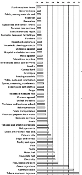
Despite being much less volatile, it might well be the case that the least volatility items in the food at home sub-group could still be more volatile than other items within the IPCA. Figure 4 tries to answer that question by listing all the 52 items that make the IPCA.34As can be seen, although the bulk of the
most volatile items do come from the food at home sub-group, many of them are not part of that club. For example, the lower volatility group mentioned above is usually placed outside the 15 most volatile items of the IPCA. In some cases they are far back on the line like beverages and “spices, seasoning, condiments and sauces”. Hence many items from the food at home sub-group can hardly be excluded based on the volatility argument.
One can also see that the three items pertaining to the energy “group” (motor fuel, household fuel and electricity) were indeed located among the most volatile items in the first period, but the situation has changed markedly ever since. For example, in the last two periods electricity was not even among the 14 most volatile items. Indeed, it was placed in 18th place in the second period and 15th in the third, hardly meritorious to be excluded based on the volatility argument. As to the household fuel item, while it was among the most volatile in the first two periods, it was displaced to the 18th position in the last period.
As explained in the last section, besides food and energy goods regulated and administered prices (several of which pertain to the energy “goods” group) are also purged from the Brazilian exclusion core. Among those, the most representative ones belong to the following items: communications, public transportation, electricity, motor fuel and household fuel. Figure 3 provides some interesting findings on their regard. First, with the exception of public transportation – which is far from being among the most volatile items in any of the three periods – the other regulated and administered prices were among the most volatile group during the first period. Second, the (relative) volatility of those prices has reduced over the sample, influenced by the decreasing volatility in the energy “goods”. Indeed, among the seven most volatile items, four came from the regulated and administered prices in the first period, two in the second period and just one (in sixth place) in the last period, which leads us to the next crucial evidence: the nature of volatility shocks presented important changes over time in Brazil, suggesting that any strategy that excludes a particular group of items could end up doing a poor job if those groups do not maintain themselves among the most volatile ones.
The evidence so far leads us to conclude that, with the exception of part of the food at home items and the “motor fuels” item, many items within the food and energy group have been excluded based on the presumption that has actually not been corroborated by the data. The same holds true for some items in the administered and regulated prices group, such as public transportation, communications and electricity. The last two were very volatile in the first period, but not in the other two.
However, it should be called to attention that volatility is not the rationale behind the removal of regulated and administered prices from the IPCA. The two main (related) arguments are:
a) those prices are not affected by monetary policy;
34Notice that three items were created in August 1999. Hence the number of items in the first sub sample is smaller; while in
b) they are not determined by market forces but rather by contracts or other factors (e.g. politically motivated).
However, these arguments seem pretty fragile.35 Moreover, even if it were true it would probably not
support their exclusion. Although monetary policy does not affect those prices in the very short run, it does affect them at longer horizons. Indeed, in Brazil regulated prices are changed on an annual basis as laid out in contracts, and since those contracts are tightly linked to past inflation they are indeed affected by monetary policy, but with a lag.36 In its turn, administered prices such as health insurance are adjusted taking heavily into account past inflation.
More crucially, since regulated and administered prices are very persistent, being rigid downwards, their changes have usually a permanent nature and, in this case, we certainly would not want to exclude them from the index, otherwise the core would be biased. Indeed, da Silva Filho (2008) calls to attention not only the diverging trends between the exclusion core index and the IPCA, reflecting the rather permanent nature of those price changes, but also the asymmetric response of regulated prices to changes in the exchange rate.
Not by coincidence, the evidence put forward in the last section showed that the exclusion and the trimmed mean cores present large biases. Indeed, in the exclusion core, administered and regulated prices are excluded by construction, and in the trimmed mean case, since those prices are changed infrequently (once a year), once the change occurs, given the large relative monthly changes, they are also “automatically” excluded.
Given the above unsatisfactory picture, a new exclusion core, with sounder statistical and economic foundations, is proposed. There are two main differences between the current and the new exclusion core (named IPCAEX1). First, the statistical foundation of the latter is stronger. More precisely: instead of just claiming that certain prices are more volatile than others, we use an objective statistical crite-rion to both select and exclude the most volatile items. Second, as argued above, we do not concur that administered and regulated prices should be purged from the IPCA, quite on the contrary, those are precisely the prices that should notbe excluded from the index, given the permanent nature of the “shocks” they are subjected to. Their exclusion was particularly harmful during periods of sharp exchange rate depreciation, such as after the floating, in 1999, and in the pre-election scare, in 2002, since their prices are strongly influenced by the exchange rate.
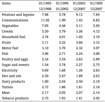
Table 5 lists all IPCA items whose relative price volatilities are above two standard deviations, during the 1995.1–2007.12 period (last column). This feature is considered to be a necessary condition, yet not sufficient, for a given item to be excluded. Sixteen items fulfilled that condition. As one can see, the list is largely dominated by food items, although energy items, regulated and administered prices and some “outsiders” (tobacco and tuition) are also present. This evidence is exactly the same one already portrayed in Figures 2 to 4.
However, items’ volatility sometimes changes radically from one period to another, as seen above. For example, although communication holds the second place overall, it was not among the most volatile in the second and third sub-periods. Hence, another desirable criterion should be consistency: the item should be consistently among the most volatile ones (in the current case for at least two out of the three sub-periods) to be excluded. This additional requirement discards the following items: communications, electricity, tuition and tobacco. In all those cases, the high overall volatility was entirely due to the high volatility observed in the first period. Moreover, both communications and electricity are regulated prices and, as argued before, should not be excluded from the index.
35Note that using this same (fallacious) reasoning one could also argue that wages are not affected by monetary policy, since
most wage contracts are set for pre-determined time periods.
36The price index that indexes most of the contracts is heavily influenced by the exchange rate, which is also affected by monetary
Table 5: IPCA: Relative volatility for selected items*
Items 01/1995 01/1999 01/2003 01/1995
12/1998 01/2002 12/2007 12/2007
Potatoes and legume 7.98 5.78 9.13 7.84
Communications 11.92 1.99 1.43 6.82
Vegetables 7.95 4.48 5.11 5.95
Cereals 5.30 3.79 3.26 4.12
Household fuel 3.78 4.01 1.05 3.19
Fruits 3.11 2.22 3.66 3.12
Motor fuel 3.10 3.70 2.32 3.07
Fish 3.96 2.71 2.24 3.00
Poultry and eggs 2.34 3.54 2.62 2.89
Sugar and sweets 1.54 3.78 2.27 2.75
Electricity 5.69 1.68 1.26 2.63
Fats and oils 2.30 3.47 1.89 2.63
Dairy products 1.90 2.04 2.50 2.19
Tuition 2.72 1.86 1.81 2.18
Meat 2.17 2.05 2.07 2.14
Tobacco products 2.75 1.93 1.41 2.05
(*) Measured by standard deviations.
Notice, however, that the household and motor fuel items – which are largely administered prices and also pertain to the energy group – ended up fulfilling the two statistical conditions for exclusion.37
Nonetheless, according to the economic reasoning above they should not be excluded. At this point some digression is necessary. Contrary to regulated prices, which are changed once a year and are very rigid downwards, one could claim that household and motor fuel should be excluded since they are likely to be very volatile as they are tightly linked to oil prices. Although this is certainly true for many countries, one should note that: first, in Brazil fuel prices are basically set by the Government and are changed infrequently. Hence they bear a high degree of persistence.38 Second, commodity prices,
especially oil prices, are often subjected to persistent trends, in opposition to fresh food prices. In this case, despite the high volatility, their exclusion is not advisable. As a result, the IPCAEX1 excludes 10 items from the headline index instead of the approximately 23 that are excluded from the actual exclusion core. Note that all the items come from the food at home sub-group. As a result, while the current exclusion core excluded, on average, 46.2% of the IPCA during the 1999-2007 period, the IPCAEX1 would have excluded just 10.6%.
Despite our theoretical preference for not excluding household and motor fuel items, we also calcu-late another core that also excludes them (called IPCAEX2), in order to check its performance relatively
37The household fuel item contains the following sub-items: coal, bottled cooking gas and town gas. The second one, which is
the most relevant in the CPI basket, is controlled by the Government, while the third one is a regulated price. The importance of the first one is negligible. The motor fuel item contains the following sub-items: ethanol, which is actually a free price, gasoline, diesel and vehicle gas. The last three are controlled by the Government (i.e. administered).
38For example, oil prices have fallen from US$ 150 just before the worsening of the sub-prime crisis in September 2007 to around
to IPCAEX1. In this case the number of excluded items rises from 10 to 12, and the average weight excluded during the 1999-2007 period rises from 10.6% to 17.3%. A final word of caution is required. Even though the IPCAEX1 and IPCAEX2 have sounder statistical and economic foundations than the actual exclusion core, the nature and size of price shocks can change from time to time as shown above, so that they could become biased as well. However, we do believe that not only they are less likely to be biased than the current exclusion core, but the bias would be smaller should it happen. This fact calls for the importance of checking periodically if the excluded items remain being the most volatile ones. Nonetheless, we believe that either the IPCAEX1 or the IPCAEX2 bear important methodological improvements over the actual exclusion core.
An alternative for mitigating such a problem is to exclude prices based on a clear and timely statis-tical criterion, rather than on their nature. This is the rationale behind the trimmed mean core, where prices are purged based solely on the relative size of their cross-section variation. However, even in that case if a certain “good” suffers persistent large price changes, it will be repeatedly excluded and the core could end up biased as well. Indeed, this is precisely what is behind the dismal performance of the trimmed mean core in Brazil. Since regulated and administered prices are changed infrequently, when the changes come they are usually large and, therefore, excluded. Hence, when the prices of those goods began to sharply increase following the large depreciations of 1999 and 2002, they be-came systematically excluded from the IPCA, and the trimmed mean core turned out to be biased. That is why the smoothed trimmed mean has a much better performance; because large monthly changes were equally split among the current and the next eleven months and, therefore, were less likely to be excluded.
Another possibility is that instead of excluding the most volatile items from the IPCA, some re-weighting scheme is applied to the index so that the most volatile items are downplayed, but not excluded. The literature lists some possibilities. One option is the so-called double-weighted index, in which the expenditure weights are multiplied by the inverse of the item’s volatility, so that the importance of the most volatile items is downplayed, and vice-versa. Another possibility is just to use the (inverse) volatility of a given item as its weight.
Hence, besides the IPCAEX1 and the IPCAEX2 two other new core measures are calculated: a double weighted core (IPCADP) and a volatility core (IPCAV). The IPCADP is calculated as follows.
πct=
n X
i=1 e
wi,tπi,t (11)
wherewei,t=
1/σi,t n
P
i=1 1/σi,t
wi,t,σi,t= j1
−1
r Pj
k=1
πi,trel
−k−π
rel i,t−k
2
, andπreli,t−k= 1
j Pj
k=1π
rel i,t−kand
πreli,t =πi,t−πt.
πtcis the core inflation at periodt,wi,tandwei,tare the (normalized) expenditure weights of each componentiof the IPCA and the associated new (double) weight at periodt andσi,t is the moving average volatility involving a window ofjmonths of the componentiat timet.
The IPCAV is calculated as follows:
πct= n X
i=1 b
wi,tπi,t (12)
wherewbi,t=
1/σi,t n
P
i=1 1/σi,t
is the (normalized) volatility weight of componentiat timet.
volatilities for each item. Finally, notice that since the performance of the IPCAV was disappointing its results are not shown.
6. EMPIRICAL RESULTS
Given the dismal performance of the current core inflation measures, one would like to know how well the new measures laid out above fare according to the three criteria described in Section 2. Table 6 provides the first assessment and the results seem encouraging. All three new measures do not have statistically significant biases. In the case of the IPCAEX1 the bias is virtually zero. The IPCAEX2 and the IPCADP show similar performances during the IT period and, although not negligible, their bias’ magnitude does not seem to be so economically relevant. Notice that during the IT period, the size of the largest bias among the new cores (0.34 p.p. from the IPCAEX2) is one third lower than the smallest bias among the current core measures (0.51 p.p. from the smoothed trimmed mean). In addition, notice that apart from the IPCAEX1 the new cores also share a tendency to underestimate headline inflation, although to a much lesser degree. Finally, when the problematic 1999–2002 period is considered all three new cores remain statistically unbiased, especially the IPCAEX1. However, the bias for both the IPCAEX2 (−1.28) and the IPCADP (−1.26) is now economically relevant.
Table 6: Descriptive statistics for IPCA core inflation measures
Measures of core inflation Monthly Standard VAriation Annual bias Unbiasedness test average deviation coefficient (p.p) (p-value)
1996-2008
Headline inflation 0.54 0.45 0.84 -
-IPCAEX1 0.55 0.41 0.75 0.09 0.88
IPCAEX2 0.52 0.34 0.65 -0.23 0.67
IPCADP 0.50 0.34 0.68 -0.48 0.38
1999-2008
Headline inflation 0.57 0.45 0.79 -
-IPCAEX1 0.57 0.39 0.69 -0.02 0.98
IPCAEX2 0.54 0.30 0.56 -0.34 0.56
IPCADP 0.55 0.31 0.57 -0.32 0.59
1999-2002
Headline inflation 0.70 0.54 0.77 -
-IPCAEX1 0.68 0.44 0.65 -0.23 0.85
IPCAEX2 0.60 0.32 0.53 -1.28 0.24
IPCADP 0.60 0.36 0.60 -1.26 0.27
trade-off between bias and variance for the ICPAEX1, the least biased among all.39 This result hinges
on its minimalist nature since it excludes, on average, only 10.6% from the IPCA, during the 1999–2008 period. Although the IPCAEX1 has our theoretical preference, the IPCAEX2 seems to deliver a better balance between bias and variance.40
Finally, notice that, during the IT period, when the MSE criterion is chosen, there is a sharp increase in “volatility” when the 37-month moving average is used as a proxy for trend inflation, in all cases. This result suggests that both the 13 and 25-month moving averages are more appropriate for proxying the “true” trend of IPCA inflation. This reflects the fact that inflation volatility during that period was large, so that the long run in Brazil is shorter.
Table 7: Deviations from trend IPCA inflation
Measures of core inflation RMSE1 MAD2
Centered moving average Centered moving average 13-month 25-month 37-month 13-month 25-month 37-month
1996-2008
IPCAEX1 0.86** 0.87* 0.87** 0.87*** 0.91** 0.92*
IPCAEX2 0.65*** 0.66** 0.67** 0.70*** 0.75*** 0.75***
IPCADP 0.70*** 0.72** 0.74** 0.74*** 0.77*** 0.79***
1999-2008
IPCAEX1 0.85** 0.86* 0.96* 0.87** 0.91* 0.90*
IPCAEX2 0.58** 0.60** 0.74** 0.65*** 0.68*** 0.66***
IPCADP 0.66** 0.67** 0.81** 0.69*** 0.70*** 0.71***
*, ** and *** indicate significance at 10%, 5% and 1%, respectively, in Diebold & Mariano’s test for predictive accuracy.
(1) Root mean square error relative to that of headline inflation.
(2) Mean absolute deviation relative to that of headline inflation.
It is worthwhile to call to attention that besides the remarkable performance of the IPCAEX1 on the bias criterion the dynamics of its bias is in accordance to what one expects from a good core measure, as Figure 5 shows. Indeed, positive and negative “errors” often alternate each other, in opposition to what happens with the IPCAEX2 and the IPCADP. This evidence could lead one to argue that in Brazil the “optimum” core would conceptually be so close to headline inflation that actual inflation would be the best “core” of itself.
This claim seems more convincing when one is reminded of the well-known difficulties in extracting the inflation noise from signal along with the pervasiveness of several kinds of economic shocks to the Brazilian economy. Both facts would favour a “minimalist core”. Such a reading shares some common elements with claims such as that of Clinton’s (2006), who argues, for Canada, that “Under the official inflation targeting regime, core inflation is not a good predictor of headline inflation, in principle or in practice.”, or yet that of Bryan and Cecchetti’s (1994), who find evidence for the U.S. that headline inflation is a better predictor of itself than the traditional ex-food & energy core.
Table 8 provides evidence on how useful the new cores are to explain headline inflation over the near future in Brazil. The main results are: first, although theR2statistics remain extremely low they
39One easy way to deal with the higher relative volatility of the IPCAEX1 is to use its moving average.
40From a theoretical viewpoint it is interesting to notice that if the optimum core inflation is indeed a minimalist one, then
increased up to 50% in comparison to the “old” cores (see Table 3), for the IPCAEX1 and IPCAEX2 cases. In both cases the smallest gains occur in the 4-quarter ahead horizon. Also, the ICPADP does not bring any improvement over the current calculated cores, according to this criterion; second, apart from the 4-quarter ahead horizon, there also appears to be some gains when regression standard errors are compared (for the IPCAEX1 and IPCAEX2 cases). More importantly, in some cases the inclusion of core inflation now produces a decrease in the sigmas.
Table 8: Goodness of fit andF-tests results
2Q ahead 3Q ahead 4Q ahead
R2 σˆ F
1 F2 R2 σˆ F1 F2 R2 ˆσ F1 F2
Headline 0.08 1.22 - - 0.07 1.43 - - 0.09 1.71 -
-inflation
IPCAEX1 0.16 1.20 0.28 0.00/0.21 0.15 1.40 0.23 0.02/0.10 0.14 1.76 0.79 0.14/0.76
IPCAEX2 0.17 1.18 0.18 0.00/0.43 0.12 1.44 0.44 0.04/0.59 0.15 1.74 0.64 0.02/0.44
IPCADP 0.12 1.21 0.37 0.00/0.05 0.09 1.46 0.64 0.00/0.40 0.11 1.77 0.83 0.36/0.89
(1) See comments on Table 3.
Indeed, in contrast to the previous results, where the sigmas actually increased, now they fell in the 2-quarter ahead horizon for both the IPCAEX1 and IPCAEX2, and in the 3-quarter ahead case for the former. Hence, the (possible) gains brought by the new cores seem to be concentrated in the 2-quarter ahead horizon, precisely when the monetary policy is less capable of affecting inflation. The above results suggest that predicting inflation at longer horizons is a tough task in Brazil, a result that has already been documented by da Silva Filho (2006).
However, notice that the evidence regarding theF-test statistics remains unchanged, in particular the conflict between the Andrews-based and Newey-West basedF-statistics and the failure of theF -tests to reject the null. As did Table 4 for the “old” cores, Table 9 provides evidence on the conflicting
F-test statistics. As before, it suggests that the Newey-West correction seems to be more successful in dealing with the effects of overlapping observations than Andrews’. It also shows – given the non negligible difference in the p-values of theF-tests in some cases – that test statistics based on that kind of correction should be regarded with care.
Table 9: Goodness of fit andF-tests results (non overlapping observations)1
Semi-annual data Annual data
R2 σˆ F
1 F2 R2 σˆ F1 F2
Headline inflation 0.06 1.45 - - 0.06 2.78 -
-IPCAEX1 0.09 1.51 0.73 0.60/0.77 0.12 2.85 0.49 0.19
IPCAEX2 0.09 1.52 0.84 0.88/0.94 0.32 2.51 0.11 0.02
IPCADP 0.09 1.49 0.57 0.35/0.58 0.06 2.93 0.98 0.98
(1) See comments on Table 4.