Health Systems Efficiency after the Crisis in the OECD Ana Beatriz Mateus D’Avó Luís 648

(1)

A Work Project, presented as part of the requirements for the Award of a Masters Degree in Economics from the Nova – School of Business and Economics

Health Systems Efficiency after the Crisis in the OECD

Ana Beatriz Mateus D’Avó Luís

648 A Project carried out with the supervision of:

Professor Pedro Pita Barros

(2)

Health Systems Efficiency after the Crisis in the OECD

Abstract

This work evaluates the efficiency position of the health system of each OECD country. It identifies whether, or not, health systems changed in terms of quality and performance after the financial crisis. The health systems performance was calculated by fixed-effects estimator and by stochastic frontier analysis. The results suggest that many of those countries that the crisis affected the most are more efficient than the OECD average. In addition, some of those countries even managed to reach the top decile in the efficiency ranking. Finally, we analyze the stochastic frontier efficiency scores together with other health indicators to evaluate the health systems’ overall adjustments derived from the crisis.

(3)

I. Introduction

The impact of the 2008 crisis on health care has heightened the need to make

appropriate investment in health quality and to reinforce financial sustainability of the

health care systems. Of particular interest is the health care systems efficiency and

health care restructurings and improvements in order to cope with the impact of the

economic crisis.

Health systems efficiency has been studied for a period before the crisis by Joumard et

al. (2010). They found that in the OECD countries higher health care expenditures did

not necessarily mean better health status. There was indeed efficiency shortage in some

countries. Based on the results, recommendations for improvements were specified for

each country’s health system.

However, it is not clear whether the budgetary constraints and health reforms resulting

from the crisis changed those findings.

The purpose of this research is to analyze how health systems efficiency in the OECD

countries have adjusted after the crisis. Answering the main question will imply

evaluating the recent relative position of each country in the OECD health system

efficiency ranking. An analysis similar to Joumard et al. (2010) was done using

2005-2011 data, for 33 OECD countries. Moreover, it is important to observe in which

aspects health care systems are doing better and in which they are doing worse than

before 2008, so that weaknesses that prevent a better performance can be identified.

The results show that several countries changed their efficiency score after the crisis.

Some of those countries that the crisis affected the most increased their relative position

in the efficiency ranking. Moreover, the results show that if all countries improve the

system performance to the level of the most efficient county, the OECD average life

(4)

This paper is structured in the following way. Section II presents some previous

empirical work in assessing health care systems efficiency, section III describes the

methodology and data which is used. Then, the health status determinants, the

efficiency results as measured by both fixed-effects estimator and stochastic frontier

approaches, the health indicators comparison by groups of countries and the change on

the health care profile of each country are presented in section IV. Finally, we present

work limitations and conclusions in section V.

II. Literature Review

As the main objective is to have a direct comparison with the work of Joumard et al.

(2008, 2010), these studies are the starting point. They calculated health care systems

efficiency scores of 30 OECD countries by two methods: fixed-effects estimator, over

the period of 1981-2003, and data envelopment analysis, using data for 2007. They

found that on average, OECD countries could increase life expectancy at birth by 2

years if all became as efficiency as the best performer. The efficiency scores were

compared with other health indicators, particularly with those reflecting the activity and

quality of the health care system.

By cluster analysis, countries were grouped, in 6 groups, based on their health care

system’s characteristics in the form of several indicators transformed from the answers

of 29 countries to the OECD Survey on Health Systems Characteristics 2009. So that,

all health indicators would be analyzed by comparing each country not only with the

OECD average, but also with its group of countries with similar health system

characteristics. It was also found that there was no health system type considerably

better than the others. The efficiency level had a higher variance within each group than

between groups.

(5)

and international system level, as well as at hospital level within countries, by taking

different approaches. The Canadian Institute for Health Information (2014) also

measured the health care efficiency and its determinants for the different regions in

Canada using data envelopment analysis. And they found that there were regional

differences in performance and that by maximizing their efficiency, regions could on

average reduce treatable causes of death by 18% to 35%. They also found that less

smoking, obesity and chronic conditions, shorter lengths of stay, more equity in health

access and more primary care investment have significant impact on regional efficiency.

Alternative approaches to measure performance of health care have been taken in other

studies. WHO (2000) and Evans et al. (2000) studied the health care system efficiency

of 191 countries for 1997, by a stochastic frontier analysis, taking the

Disability-Adjusted Life Expectancy as health status of the population. Murray and Evans (2003)

pointed out that the stochastic frontier analysis is more appropriate in efficiency

measurement than the data envelopment analysis, since the latter method attributes all

the distance to the frontier as inefficiency, not taking into account random factors.

Jourmard et al. (2008) created a health production function and found that health

spending is the factor that affects the most the health status of a population, followed by

education. They found that a 10% increase in health spending increases life expectancy

at birth by 3 to 4 months, keeping everything else constant. On the other hand, Thornton

(2002) presented empirical evidence for the USA that socioeconomic status, such as

education, income and married households have more impact on the health status of the

country, in this case, age-adjusted death rate, than health spending.

III. Data and Methodology

Given that it was not feasible to use the exact same variables as in Joumard et al. (2008,

(6)

was removed from the original model of Joumard et al (2008, 2010). The efficiency was

estimated by two approaches: 1) regressions using panel data and estimated by

fixed-effects and 2) stochastic frontier analysis, SFA (as opposed to data envelopment

analysis that was used in the above-mentioned literature). Moreover, three OECD

countries, Estonia, Israel and Slovenia were not analyzed by Joumard et al. (2008,

2010), but they are included in this paper.

Similarly to the work of Joumard et al. (2010), the efficiency scores were analyzed

together with those indicators that reflect the quality of preventive and out-patient care

sectors (vaccination, avoidable hospital admission and acute myocardial infarction and

stroke fatality rates), the hospital output efficiency (in-patient average length of stays,

acute care occupancy and turnover rates, cataract surgeries and consultations per

doctor), equity in health status, amenable mortality rates (those deaths due to causes that

could potentially be avoided with the effective treatment at the right time) and

administration costs, which are useful to assess the health system efficiency of each

country. Other indicators included in the country profiles are related to health care

prices and spending per capita and to GDP, number of health professionals and their

respective income, hospital physical resources (high-tech equipment and hospital beds),

hospital activity (doctor consultations per capita, hospital discharges and some surgery

procedures), pharmaceutical consumption, nature of health care financing (public,

private insurance, of-pocket) and spending destination sectors (in-patient,

out-patient, medical goods). All these indicators (Table 1) were not considered as inputs in

the health production function, because these indicators are hospital’s output-based

efficiency indicators. Yet they are a complement in the study of the system

(outcome-based) efficiency determinants.

(7)

developed by calculations for this paper. For comparison purposes, the same proxy for

health status equity was calculated as in Joumard et al. (2010), by the inverse of the

standard deviation in the age of death for population aged above 10, using data on

number of deaths by age from the Human Mortality Database. This age dispersion was

proposed by Edwards and Tuljapurkar (2005) as a proxy for health inequalities in health

status. An output efficiency indicator, the acute care turnover rate, was also calculated,

by dividing the number of acute discharges by the number or available acute care beds.

Table 1 - Health care indicators by area

Efficiency and quality Amenable mortality

 SFA efficiency score

 Equity score

 Average length of stay

o_{All in-patient; Colorectal cancer; Lung cancer; Breast} cancer; Acute myocardial infarction; Femur fracture

 Acute occupancy rate

 Acute turnover rate

 Cataract surgery

 Consultations per doctor

 Expenditure in health administration

 Vaccination rates

o_{Diphtheria, tetanus and pertussis; Measles; Influenza}

 Avoidable hospital admission rates o_{Asthma; Bronchitis; Heart Failure}

 In-hospital case fatality rates

o_{Acute myocardial Infarction; Ischemic stroke}

 All causes

 Infectious diseases

 Cancers

 Endocrine, nutritional and metabolic diseases

 Diseases of nervous system

 Diseases of circulatory system

 Diseases of genitor-urinary system

 Diseases of respiratory system

 Diseases of digestive system

 Perinatal mortality

Prices and physical resources Activity and consumption Financing and spending

 Total health expenditure

 Practicing physicians

 Practicing nurses

 Medical graduates

 MRI units

 Computed tomography scanners

 Number of acute care beds

 Remuneration of hospital nurses

 Remuneration of general practitioners

 Remuneration of specialists

 Relative health prices to GDP

 Doctor consultations

 Hospital discharges

 Hip replacement

 Knee replacement

 Appendectomy

 Caesareans sections

 Antidepressants

 Anxiolytics

 Analgesics

 Anti-inflammatory, antirheumatism

 Antibacterials for systemic use

 Cardiovascular system

 Drugs for diabetes

 Public spending

 General government funding

 Social security funding

 Private health insurance funding

 Out-of-pocket payments

 Expenditure on medical goods

 Expenditure on out-patient care

 Expenditure on in-patient

 Expenditure on collective services (public health services and health administration)

Source: Joumard at al. (2010)

To calculate the efficiency of the health systems, a production function was designed for

the health care at the system level.

The production function’s output and input data were retrieved from OECD Health Data

(8)

and 2011, for the majority of the variables. The purpose was to get as many years before

as after the financial crisis of 2008.

As the output at the system level, life expectancy at birth, for females, males and both,

and life expectancy at age 65 for each gender were the variables used as proxy for the

health status of each countries’ population. Life expectancy at birth for both genders

was considered the dependent variable for the efficiency calculations, by both

fixed-effects estimator and stochastic frontier approaches. Other proxies could be thought as

more desirable as one assumes that it is important to take into account the quality of life

of the population (Joumard et al., 2008). However, regarding all possible health status

indicators, longevity data was the most complete one.

Health status depends on the quantity of medical care services that is offered to the

population, thus the variable used as its proxy was total health expenditure per capita

US$ PPP rates. Moreover, the health care that the population receive over the years also

influence the current health status. Therefore, a variable with the cumulative value of

health investment was also considered as a variable of health stock of the previous three

years. It has been debatable whether a discount rate for healthcare should be taken into

account, and at what value (Acharya and Murray, 2003; Stahl, 2004), therefore the

ad-hoc discount rate of 10% was chosen.

Two population’s lifestyle indicators (alcohol and diet) were used as control variables in

the fixed-effects estimator. Alcohol consumption in liters per capita was introduced as a

1-year lag variable, as the current level of alcohol consumption may have an impact in

health status, but alcohol data for all countries is only complete until 2010. A proxy for

diet, consumption of fruits and vegetables in kilograms was also taken into account in

the production functions.

(9)

not possible to do it since ten of the thirty-four OECD countries could not be analyzed.

Data for tobacco consumption in grams per capita is nonexistent for Chile, Estonia,

Luxembourg, Mexico, Slovakia and Slovenia and is missing for several other countries,

either in recent years or in lagged values. Other alternative measures of tobacco

consumption (e.g. share of daily smokers; number of cigarettes smoked per day) also

present missing data for many countries.

The exogenous variables’ set also included one environmental factor affecting

population’s health: emissions of nitrogen oxide in kilograms per capita. This factor

represents air pollution in each country which especially affects the respiratory system,

and so may affect life expectancy.

Education and income are the two socioeconomic variables taken into account in the

models. The education variable is measured by the share of adult population with at

least upper secondary school. Income is measured by the GDP per capita US$ PPP rate.

The regressions by fixed-effects estimator were the first approach used to calculate the

efficiency ranking,1 allowing for a direct comparison with Joumard et al. (2008, 2010).

And were also the main approach used to verify the impact of health expenditure on the

health status of the population of each country, while controlling for other lifestyle and

socioeconomic variables (alcohol consumption, diet, pollution, education and GDP).

Life expectancy at birth for females, males and both, and life expectancy at age of 65

for females and males were the dependent variables for the analysis of impact of each

independent variable. However, to get the efficiency score only life expectancy at birth

for total population was taken as the dependent variable. Moreover, all variables

included in the regressions were transformed in logarithms.

The assumption of this method by fixed-effects estimator is that what is not accounted

1

(10)

for by the model reflects the health care system efficiency of the country (Joumard et

al., 2008). This efficiency score was calculated by adding up the country fixed-effects to

the residuals of the latest year in study. This sum measures the distance to the

production frontier. Thus, it was assumed that the country fixed-effects are part of the

country inefficiency, and are not revealing a different production frontier for each

country.

The alternative methodology of this paper to calculate the inefficiency score is the

Stochastic Frontier Analysis (SFA).2_{The frontier is the maximum outcome (health}

status) that is possible to reach given the level of inputs in use. This method allows to

make the distinction between the part of the residual that is due to random factors and

the part of the residual that accounts for the country inefficiency. The production

function used was the same one as in the regressions with fixed-effects estimator

referred above. The same output and inputs transformed in logarithms were included.

Modeling the production frontier with panel data increases the number of observations

and accuracy of estimates. This way, it is feasible to calculate the system inefficiency by

analyzing the frontier with country fixed-effects incorporated into the inefficiency

equation, which is compatible with the previous approach by fixed-effects estimator.

Besides, with a stochastic frontier model using fixed-effects there is no need to make

any assumptions about the inefficiency term’s distribution, which makes this method

less restrictive (Murray and Evans, 2003).

Although the efficiency was calculated for 2011 by both methods, there were two

exceptions that had different latest years available: for Korea and Mexico the score was

calculated for 2010 and 2008, respectively.

2_{Coelli, Timothy J., D.S. Prasada Rao, Christopher J. O'Donnell, and George E. Battese. (2005).}

(11)

For Chile, education data is missing for 2005 and 2006 and data of nitrogen oxide

emissions is missing for the rest of the studied years, therefore it is the only OECD

country not being analyzed here.

In this work it was assumed as reasonable to compare efficiency scores and other health

indicators within and across the group of countries with similar health care system

characteristics that are resulting from the Survey on Health Systems Characteristics

2008-2009 analysis made by Joumard et al. (2010). Although there is some new data for

countries’ health policy and institutions, from the Survey on Health Systems

Characteristics 2012, this data was not as complete. More recently, other authors (e.g.

Pisu, 2014 and Tchicaya and Lorentz, 2014) analyzed health care sectors and systems

using the indicators of system characteristics that result from Joumard et al. (2010) and

other data from the Survey on Health Systems Characteristics 2008-2009.

IV. Results

The economic crisis in mid-2008 had a visible impact on the OECD average health

spending per capita, US$ PPP. On average the health spending growth decreased after

2008, especially between 2009 and 2010 when the average growth rate was close to

zero. However, some countries actually decreased their total health spending per capita

after the crisis, namely Czech Republic, Estonia, Greece, Iceland, Ireland, Portugal,

Slovak Republic, Slovenia, Spain, Turkey and United Kingdom. Some of those still had

negative health spending growth in 2011: Greece, Ireland, Portugal, Slovak Republic

and Spain (Morgan and Astolfi, 2014).

Now we know how the main health sector input evolved, therefore it is important to

understand the impact of this and other non-health sector inputs on the health status, as

well as, what happened to the efficiency of these countries individually.

IV.1 Health status determinants

(12)

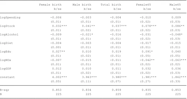
standard errors.3

Table 2 indicates that a country has higher life expectancy at birth of total population if

it spends more in health care, has more adults with at least upper secondary education

and less air pollution. These coefficients are statistically significant, at the 1% or 5%

level, for life expectancy at birth of total population, i.e. for both female and male.

Table 2– Fixed-effects estimator output: Health status determinants

The variables’ coefficients in the regressions have the expected signs. The exception is

the coefficient for diet, consumption of fruits and vegetables, which has a negative

impact in health status. However its impact is not statistically significant.

In this period of 2005-2011, the regressions output reveal that for total population

income per capita and the lifestyle variables, alcohol and fruits and vegetables

consumption, are not significantly different from zero and that education is the variable

with the highest elasticity. This may be due to higher education meaning more access to

health information and a better understanding of it by the patients which may have

impact on the efficacy of medical services (Thornton, 2002). Nevertheless, the OECD

3

There may be some endogeneity effect, as the level of total healthcare expenditure is a function of the income level. Table A.2 in appendix shows that by excluding the variable of GDP in the fixed-effects estimator regressions, the coefficient of health spending increases, suggesting that the variable of spending includes the income effect not related to health, which may lead to biased estimators. For this reason and for the lack of reliable instrumental variables, Joumard et al. (2008) included both health spending and GDP variables in their model. In this paper, we also included them for comparison reasons.

* p<0.10, ** p<0.05, *** p<0.01

(13)

average of life expectancy at birth of total population may increase 2.86 months if the

average spending increases by 10%, keeping everything else constant.

Table A.3 in appendix presents another specification of the model including a variable

of health stock. However, the stock of investment in health is highly correlated with the

current health spending (Table A.4 in appendix). Thus, the variable of health stock was

not included in the main model of efficiency measure.

IV.2 Fixed-effects estimator – Efficiency ranking

By taking life expectancy at birth for total population as the dependent variable, the

fixed-effects and the residuals specify the years of life gained or lost compared to those

years of life expectancy that were expected if the country had the same efficiency as the

OECD average. Which means that, by these assumptions, Austria has the average

efficiency, while Spain’s high efficiency allows it to get 4 more years compared to the

(average) output that was expected by the model. On the other hand, the United States

of America is the OECD country with the least efficient healthcare system, according to

the fixed-effects estimator method, losing 4 years of life expectancy compared to the

expected output. Figure 1 presents these deviations in years of life expectancy at birth

for total population, resulting in the ranking of countries’ health system efficiency.

Figure 1 - Country fixed-effects and residuals deviation from OECD average, 2011: Years of life expectancy not accounted for by the model (Fixed-effects estimator)

(14)

Comparatively to the 2003 efficiency results from Jourmard et al. (2008, 2010),

measured by fixed-effects estimator under the same assumptions (Figure A.1 in

appendix), it is possible to notice that, for 2011, there were some changes on the relative

position of this efficiency ranking. The results displayed in Figure 1 indicate that, taking

into account only those 23 countries studied by fixed-effects estimator in Joumard et al.

(2008, 2010), Poland and Sweden went down considerably in the ranking, while United

Kingdom and Austria became more efficient than the average.

IV.3 Stochastic Frontier Analysis – Efficiency scores

By the second method, the stochastic frontier analysis, the resulting inefficiency scores

were converted into years of life expectancy that the country can potentially gain if it

increases its efficiency to the level determined by the frontier (Table A.5 in appendix

shows the SFA coefficients). By incorporating country fixed-effects into the model,

typically one or more countries are in the frontier and assumed as being totally efficient,

while the other countries are analyzed by comparison to those efficient ones

(Kumbhakar and Lovell, 2000).

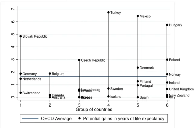
Figure 2 - Potential gains in years of life expectancy (Stochastic Frontier Analysis)

In this case, the countries that are completely efficient are, Japan, Spain, Greece, Korea

and Australia, their observed output is placed on the production frontier. While Turkey,

Mexico and Hungary could increase their total population life expectancy at birth by

approximately 6 years if they were as efficient as the most efficient countries.

(15)

IV.4 Fixed-effects estimator vs Stochastic frontier

For the calculations of the potential gains in life expectancy by both methods, the

reference is the most efficient country. These scores result from comparing each country

with the most efficient one.

Figure 3 - Potential gains in years of life expectancy at birth: Fixed-effects estimator and Stochastic Frontier analysis plot

Although there are some changes on efficiency ranking places, the results are similar in

terms of which countries are the most efficient ones and which ones are the least

efficient (Figure 3). However, the maximum number of years a country can potentially

increase its life expectancy is 1 year lower by the stochastic frontier method than by the

fixed-effects estimator method. Additionally, by the stochastic frontier analysis, the

potential gains of life expectancy at birth are, on average, 1 years and 8 months, but by

the fixed-effects estimator, the average potential gains is 3 years and 8 months.

From those countries with negative health spending growth in 2011, Spain, Portugal,

Greece and Ireland have above OECD average efficiency, while Slovak Republic is the

only one which has below average efficiency, as measured by both efficiency

Australia

Austria Belgium Canada

Czech Republic DenmarkEstonia Finland

France

Germany

Greece

Hungary

Iceland

Ireland Israel

Italy Japan

Korea

Luxembourg

Mexico Netherlands

New Zealand

Norway Poland

Portugal

Slovak Republic

Slovenia

Spain

Sweden Switzerland

Turkey

United Kingdom

United States

0

2

4

6

8

0 1 2 3 4 5 6 7

Stochastic Frontier Analysis

(16)

approaches.

IV.5 Changes within and across groups

From those six groups of countries with similar health systems characteristics resulting

from the work of Joumard et al. (2010),4_{the same analysis comparing efficiency scores,}

as measured by the stochastic frontier, within and between groups was done. The

analysis showed that there are efficient and inefficient countries (above and below

OECD average efficiency) in every group (Figure 4). Moreover, as presented in Table 3,

the number of years of life expectancy a country could gain by increasing its efficiency

to the frontier level has higher variance within groups than between groups. These

conclusions correspond to the results for 2007, from Joumard et al. (2010), emphasizing

once again that no health system type has necessarily better performance than the

others.

From the 2011 results in Figure 4 and Table 3, it is possible to compare the 2007 results,

presented in Figure A.2 in appendix, from similar work done by Jourmard et al. (2010).

Yet, some OECD countries which efficiency was analyzed for 2011, can still not be

included in the analysis of this section. This is the case of Estonia, Israel, Slovenia and

United States of America, since they did not participate in the Survey on Health

Systems Characteristics 2008-2009, therefore it was not possible to group them for their

health system characteristics like the other countries.

Within group 1 (Germany, Netherlands, Slovak Republic, Switzerland), only the

4

Group 1 is composed by countries that rely on market mechanisms at the provider level and a high share of private basic insurance.

Group 2 is composed by countries that rely on market mechanisms at the provider level, public basic insurance, private over-the-basic insurance and gate-keeping.

Group 3 is composed by countries that rely on market mechanisms at provider level, public basic insurance, little private over-the-basic insurance and no gate-keeping.

Group 4 is composed by countries that rely mostly on public provision and insurance, no gate keeping and wide choice of providers.

Group 5 is composed by countries that rely on public provision and public insurance, gate-keeping, limited choice of providers and soft budget constraint.

(17)

Netherlands’ efficiency score shifted to above average, but the group mean efficiency

after the crisis is still worse than the OECD average. Switzerland still has the highest

efficiency, while the least efficient country is represented by Slovak Republic.

Figure 4 - Potential gains in life expectancy at birth across and within country groups plot (Stochastic Frontier Analysis)

Table 3 - Potential gains in life expectancy at birth within and across groups: mean and variance (Stochastic Frontier Analysis)

Group of countries with similar system characterisitics

Potential gains in years of life expectancy Mean Variance

1: Germany, Netherlands, Slovak Republic, Switzerland 2,1 3,7

2: Australia, Belgium, Canada, France 0,6 0,8

3: Austria, Czech Republic, Greece, Japan, Korea, Luxembourg 0,7 1,3

4: Iceland, Sweeden, Turkey 2,5 13,6

5: Denmark, Finland, Mexico, Portugal, Spain 2,2 6,4

6: Hungary, Ireland, Italy, New Zealand, Norway, Poland, United Kingdom 1,8 4,1

Total 1,6 3,9

Intra-group - 4,4

Inter-group - 0,5

Group 2 (Australia, Belgium, Canada, France) has seen some small changes where

Canada and France improved their performance and are now in quite high and very

close relative positions. Yet, Australia and Belgium are still the most and the least

Australia Austria Belgium Canada Czech Republic Denmark Finland France Germany Greece Hungary Iceland Ireland Italy Japan Korea Luxembourg Mexico Netherlands New Zealand Norway Poland Portugal Slovak Republic Spain Sweden Switzerland Turkey United Kingdom 0 1 2 3 4 5 6 7

1 2 3 4 5 6

Group of countries

(18)

efficient countries, respectively. This group keeps having a better mean performance

than the OECD average and has now the highest performance among the groups.

The third group (Austria, Czech Republic, Greece, Japan, Korea, Luxembourg) had

efficiency improvements in general, especially the major increase of Greece’s

efficiency, that in 2011 is the highest of the group together with Japan and Korea.

Austria is also performing well and Luxembourg improved and is now very close to

Austria’s efficiency level. The worst performer of this group is now Czech Republic

that keeps below average after the crisis.

The forth group, composed by Iceland, Sweden and Turkey, had the highest mean

efficiency, in 2007. However, it has now a lower mean efficiency and is the group with

the highest score variance. Iceland and Sweden continue performing well, however after

the crisis, Turkey had a great decrease of performance and goes from the highest to the

lowest efficiency score of this group.

Concerning group 5 (Denmark, Finland, Mexico, Portugal, Spain), Spain and Portugal

continue to have high efficiency levels and Finland has improved its performance since

2007. Denmark is still performing below the OECD average. Mexico has the most

extreme change of position as it goes from being the most efficient country to the least

efficient one of the fifth group. This leads to a low group mean efficiency.

The countries of group 6 (Hungary, Ireland, Italy, New Zealand, Norway, Poland,

United Kingdom) are still performing worse than the OECD average. Although Italy

and Hungary continue being the highest and the lowest performers, respectively, there

were some shifts in this group after the crisis. In 2011, Ireland, United Kingdom and

New Zealand have above average scores, while Norway and Poland are performing

worse than before.

(19)

comparing them with the OECD average and with the previous results measured by data

envelopment analysis (Figure A.2 in the appendix) from Jourmard et al. (2010), it is

possible to verify that, after the crisis, most of those countries with high or low

efficiency keep similar relative positions. Moreover, Spain and Italy became even more

efficient than in 2007. Nevertheless, some other countries changed from their inefficient

situation and became more efficient than the average, namely Greece, Ireland, New

Zealand, Austria, Finland, Netherlands Luxembourg and United Kingdom. While

Mexico, Turkey, Poland and Norway decreased their position and became inefficient.

IV.6 Other health indicators – group comparison

On average, the inequalities in health status, measured by the standard deviation of the

age of death for population aged above 10, increased almost 1 standard deviation after

the crisis (Figure 5). The group with the lowest average of inequalities is now group 1,

composed by Germany, Netherlands, Slovak Republic and Switzerland. While group 2

still has on average the highest level of inequalities. Comparatively to 2007, there were

some changes within groups. In group 1, the country with the highest level of

inequalities continues to be Slovak Republic, however the one with the lowest level is

now Germany. In 2011, group 2 has Australia as the country with the most inequalities

and Belgium with the lowest. In group 3, Luxembourg became the country with the

highest inequalities, however, Japan passed from having the highest level to the lowest

of the group. In group 4 it is now possible to notice the highest within group variation,

between the high level of inequalities of Iceland and the low level of Sweden. Group 5

appears as the only group without changes in inequalities ranking. While in the sixth

group, Italy keeps having the lowest inequality levels, but Ireland became the country

with the highest level.

In 2011, the OECD average life expectancy at birth is 80 years (Figure 6). With the

(20)

higher than the OECD average, every group have wide within variations, since they

include countries with both above and below average life expectancy.

Figure 5 - Inequalities in health status across country groups of health system characteristics, 2011 (or latest year available)

Source: Human Mortality Database.

Figure 6 - Total population life expectancy at birth across country groups of health system characteristics, 2011 (or latest year available)

Source: OECD Health Data 2014.

Figure 7 - Total Health expenditure per capita, US$ PPP across country groups of health system characteristics, 2011 (or latest year available)

Figure 8 - Administrative costs across county groups of health system characteristics, 2011 (or latest year available)

12 14 16

DEU NLD SVK CHE

Gro

u

p

1

AUS BEL _CAN FRA

Gro

u

p

2

AUT CZE GRC JPN KOR LUX

Gro u p 3 IS L S WE _TUR Gro u p 4 DNK F IN M

EX _PRT _ESP

Gro

u

p

5

HUN IRL ITA NZL NOR POL GBR

Gro

u

p

6

Inequalities OECD average

73 78 83

DEU NLD SVK CHE

Gro

u

p

1

AUS BEL _CAN FRA

Gro

u

p

2

EX _PRT _ESP

Gro

u

p

5

Gro

u

p

6

Life expectancy at birth OECD average

0 2000 4000 6000 DE U NL D S VK CHE Gro u p 1

AUS BEL _CAN FRA

G

ro

u

p

2

Gro u p 3 IS L S

WE _TUR

Gro u p 4 DNK F IN M

EX _PRT _ESP

Gro

u

p

5

Gro

u

p

6

Total Health Expenditure per capita, US$ PPP OECD average

0 2 4 6 8

DEU NLD SVK CHE

Gro

u

p

1

AUS BEL _CAN FRA

Gro

u

p

2

EX _PRT _ESP

Gro

u

p

5

Gro

u

p

6

(21)

Total health expenditure per capita continues to be higher on average in groups 1 and 2.

The forth group has the lowest spending on average, with contribution of Iceland’s great

health expenditure decrease in 2010 (Figure 7).

In general, in 2011 the OECD average administrative costs in percentage of total health

spending decreased. The countries that in 2007 had this percentage much higher than

the average decreased it considerably after the crisis. For instance, Luxembourg had the

second highest percentage of administration costs before, however, it is now among the

countries with the lowest percentage (Figure 8).

IV.7 Health indicators comparison between 2007 and 2011

To complement the countries’ profile, the stochastic frontier efficiency scores were

analyzed together with other health indicators. In this section, we compare the recent

levels of the health indicators with those 2007 levels studied by Joumard et al. (2010).

In Table 4, we compare each country against the OECD average, pointing out the main

changes occurring after the crisis. Some of the recommendations presented in the

previously referred work were taken into account to verify whether they were followed

by the countries or not. Moreover, we present the potential total health savings per

capita, US$ PPP, for the countries that are not totally efficient. The potential health

savings were estimated by the change on health spending that leads the country to the

efficiency frontier, keeping the same life expectancy level and the other inputs constant.

The health care indicators are divided by areas, the same ones as those in Joumard et al.

(2010): efficiency and quality; amenable mortality; health prices and physical resources;

activity and consumption; financing and spending.

Besides a high efficiency score, one would consider the ideal health care system as the

one having low inequalities in health status, low amenable mortality rates, low

administrative costs, short average length of stay, high quality of service provision, an

(22)

balanced share of resources between sectors.

Table 4– Main changes on countries’ profile and potential health savings per capita

Country (SFA Rank) Efficiency and quality; Amenable mortality Prices and physical resources Activity and consumption Financing and spending Previous recommendations status;

Potential total health savings/ capita (US$ PPP)5

Australia (5) High efficiency; Higher inequalities; Shorter in-patient stays; Mixed quality More doctors, nurses and medical students; Lower prices More hospital discharges Achieved:

- Reducing length of stay of in-patient care Austria (13) Higher efficiency; Longer stays; More consultations/ doctor Higher prices Low pharmaceuticals consumption/ capita Higher spending share on out-patient care

Not achieved: - Increasing quality Not totally achieved: - Rebalancing in-patient and out-patient resources Potential savings: 1198.15$ (25.7% of health spending)

Belgium (24) Low efficiency; Less inequalities; More consultations/ doctor Less doctors and nurses; Higher income of health professionals Not achieved:

- Increase hospital efficiency; - Reducing number of doctor consultations;

- Reducing administrative costs Potential savings: 2782.79$ (65.8% of health spending)

Canada (9) High efficiency; High inequalities; More consultations/ capita; Low pharmaceuticals consumption Not achieved: - Reducing inequalities

Czech Republic (26) Low efficiency; Lower amenable mortality; Long stays More students; Above average income of general practitioners Higher spending on out-patient care Not achieved:

- Reducing number of doctor consultations;

- Improving quality Potential savings: 1667.58$ (82.2% of health spending)

Denmark (25) Low efficiency; Less consultations/ doctor; Less inequalities More scanners High income of general practitioners Less consultations/ capita Achieved:

- Decreasing the excessive demand to general practitioners Potential savings: 3358.31$ (73.9% of health spending)

Estonia (27) Low efficiency; Low equity; Low amenable mortality; Low hospital efficiency; Low quality of care Few human and physical resources; Very low remuneration of health professionals Low hospital activity; Low pharmaceuticals consumption Low spending on in-patient; High spending on out-patient and on medical goods

Potential savings: 1126.79$ (83% of health spending)

Finland (20) Higher efficiency; Lower amenable mortality; Low in-patient efficiency More medical students Achieved:

- Increasing spending share on out-patient care

Not achieved:

- Decreasing inequalities; - Improving out-patient care quality

5

(23)

Potential total health savings/ capita (US$ PPP)5 Potential savings: 1777.20$ (51.4% of health spending)

France (10) High efficiency; Higher amenable mortality; Shorter stays Low remuneration of health professionals Higher pharmaceuticals consumption Not achieved:

- Decreasing health status inequalities;

- Reducing administrative costs

Germany (23) Low efficiency; High equity; Higher amenable mortality; More consultations/ doctor, but lower hospital efficiency More consultations/ capita Not achieved:

- Adjusting policies to avoid excessive hospital activity Potential savings: 3023.68$ (65.6% of health spending)

Greece (3) Higher efficiency; Lower amenable mortality; Low administrative costs Few consultations/ capita; More hospital discharges Higher spending on in-patient care; Low spending on out-patient care Hungary (31) Low efficiency; Less inequalities; Lower amenable mortality; Low hospital efficiency Achieved:

- Decreasing inequalities Not achieved:

- Rebalancing resources from medical goods to in-patient and out-patient care

Potential savings: 1744.54$ (96.9% of health spending)

Iceland (7) High efficiency; More inequalities; Short stays; Lower preventive care quality Lower remuneration of nurses and general practitioners Lower spending to GDP; More spending on medical goods and on out-patient care

Not achieved:

- Control health care spending; - Reducing spending on in-patient care;

- Reducing number of human resources and increase quality of care Ireland (19) Higher efficiency; More inequalities; Lower amenable mortality Less doctors; Higher income of nurses Few consultations/ capita Lower public spending

Israel (11) High efficiency; Low equity; Low amenable mortality; Rather high hospital efficiency Few physical resources; More doctors; High income of nurses; Low health prices High private health insurance and out-of-pocket financing

Potential savings: 198.82$ (9% of health spending)

Italy (6) High efficiency; Higher amenable mortality; Rather low hospital efficiency Below average remuneration of nurses and specialist

Not achieved:

- Improving efficiency on the in-patient care sector Potential savings: 6.17$ (0.19% of health spending)

Japan (1) High efficiency; Higher amenable mortality; High equity; Higher spending to GDP Not achieved:

(24)

Potential total health savings/ capita (US$ PPP)5 Higher

preventive care quality

consultations Partially achieved: - Improving quality Potential savings: 490.47$ (14.2% of health spending)

Korea (4) High efficiency; Higher preventive care quality Not achieved:

- Reducing the number of doctor consultations Luxembourg (14) Higher efficiency; Mixed quality; Lower administrative costs Not achieved:

- Improving in-patient care efficiency;

- Increasing out-of-pocket payments

Achieved:

- Reducing administrative costs Potential savings: 1353.62$ (29% of health spending)

Mexico (32) Lower efficiency; High amenable mortality; Short stays; Rather low quality of care

Lower prices Few hospital discharges Lower spending on medical goods; Very low spending on in-patient care Not achieved:

- Improving health status of the population;

- Reducing administrative costs Potential savings: 861.82$ (98.3% of health spending)

Netherlands (21)

Average efficiency

New Zealand

(8) Higher efficiency

Less hospital beds; Higher income of specialists Less consultations/ capita Not achieved:

- Reducing inequalities; - Reducing high administrative costs;

- Improving hospital efficiency Potential savings: 313.51$ (9.9% of health spending)

Norway (22) Lower efficiency; Few consultations/ doctor Less nurses Few consultations/ capita Not achieved:

- Reducing number of doctors for the needs of the population Potential savings: 3695.81$ (64.3% of health spending)

Poland (28) Lower efficiency; Lower amenable mortality; Longer stays; Below average remuneration of health professionals Less hospital discharges Not achieved:

- Decreasing inequalities; - Increasing hospital efficiency; - Increasing quality of care Potential savings: 1239.46$ (82.9% of health spending)

Portugal (18) High efficiency; Less inequalities; Lower amenable mortality More medical students/ capita Lower public spending Not achieved:

- Improving efficiency of in-patient sector;

- Increasing number of consultations/ doctor; - Improving quality of care Potential savings: 1102.35$ (41.7% of health spending)

Slovak Republic (30) Low efficiency; Lower amenable mortality; Rather low quality of care

Not achieved:

- Increase remuneration of health professionals to increase quality of care

Slovenia (17) High efficiency; High equity; Low amenable Few human and physical resources; Low health spending/ capita; More hospital High social and private insurance;

(25)

Potential total health savings/ capita (US$ PPP)5 mortality Low health

prices; High income of general practitioners discharges; Low pharmaceuticals consumption High spending share on in-patient and medical goods Spain (2) High efficiency; Rather high amenable mortality; More administrative costs Higher health prices; High income of nurses Not achieved:

- Improving hospital efficiency

Sweden (16) High efficiency; Higher preventive care quality Less medical students Partially achieved: - Improving quality Not achieved:

- Reducing number of doctors for the low number of doctor consultations

Switzerland (12) High efficiency; High administrative costs Lower health care prices Achieved:

- Containing health care prices Potential savings: 852.24$ (15% of health spending)

Turkey (33) Lower efficiency; High amenable mortality; Mixed quality High remuneration of health professionals More consultations/ capita; More hospital discharges Higher public spending Not achieved:

- Containing level of public health spending

United Kingdom (15) Higher efficiency; Higher amenable mortality Lower remuneration of general practitioners High pharmaceuticals consumption Not achieved: - Improving quality Potential savings: 1016.29$ (31.6% of health spending)

United States of America (29) Low efficiency; Very high amenable mortality; High administrative costs More high-tech equipment Very high spending/ capita; Less consultations and discharges/ capita High private insurance financing; Low spending on out-patient care

Source: OECD Health Data 2014; Human Mortality Database; Joumard et al. (2010)

V. Conclusions and Limitations

The levels of adult education and of health expenditure are highly associated with the

health status of the population. Keeping everything else constant, a ten percent increase

on the OECD average of total health expenditure increases life expectancy at birth of

total population by almost 3 months, on average.

The economic crisis has appeared for many countries as a challenge for the health care

(26)

increasing the same level of quality and coverage of health care services. Therefore, the

crisis was an opportunity to create reforms that changed several health care systems

efficiency. Six OECD countries, Greece, Ireland, Austria, New Zealand, United

Kingdom, Finland, Netherlands and Luxembourg increased their position relative to the

average, while four countries, Norway, Poland, Mexico and Turkey decreased it.

Southern European countries, like Spain and Greece, economies where the crisis had a

great socioeconomic impact and where expenditure controls were essential, show up as

countries that reached the top health care system efficiency. Although, these countries

decreased the total health spending per capita after the crisis, there was no immediate

effect on the health status of their population. Nevertheless, if all countries increase

their efficiency to the efficiency level of the best performer, the OECD average life

expectancy at birth of total population can still increase by almost two years.

However, the non-inclusion of tobacco consumption, due to lack of data, on the health

production function can have some efficiency implications. This can be especially

challenging in the fixed-effects estimator approach, since the assumption of including

the residuals in the efficiency score disregards the possibility of measurement errors or

other random factors.

Moreover, both methods of efficiency calculation, imply the comparison of the

countries to the best performing country. Though, the best health system derived from

the calculations does not necessarily have the best achievable performance in theory.

This means that the efficiency scores are overestimated and the top performer can

improve and reach even higher levels of efficiency and quality in the health care.

However, higher accessibility of health data, namely lifestyle and quality indicators

would improve the precision of the estimates and allow a better understanding of

(27)

VI. References

Acharya, A., and Christopher JL Murray. (2000). "Rethinking discounting of health benefits in cost effectiveness analysis." Goodness and Fairness: Ethical Issues in Health Resource Allocation. Geneva: World Health Organization.

Cameron, A. Colin, and Pravin K. Trivedi. (2005). “Linear Panel Models: Basics”

Microeconometrics: methods and applications, 697-726. Cambridge University Press.

Canadian Institute for Health Information. (2014). Measuring the Level and Determinants of Health System Efficiency in Canada. Ottawa, ON: CIHI.

Coelli, Timothy J., D.S. Prasada Rao, Christopher J. O'Donnell, and George E. Battese. (2005). “Stochastic Frontier Analysis”. An introduction to efficiency and productivity analysis, 141-61. New York: Springer.

Evans D., Tandon A., Murray C., and Lauer J. (2000). “The Comparative Efficiency of

National Health Systems in Producing Health: An Analysis of 191 Countries.”

World Health Organization, GPE Discussion Paper, No. 29.

Ferrier, G.D. (2014). “The "usefulness" of stochastic frontier analysis for health care”,

Economics and Business Letters, 3(1): 27-34.

James Thornton. (2002). “Estimating a health production function for the US: some new

evidence”, Applied Economics, 34:1, 59-62.

Joint Research Centre-European Commission. (2008). Handbook on constructing composite indicators: methodology and user guide. OECD Publishing.

Joumard, I., C. André and C. Nicq. (2010). “Health Care Systems: Efficiency and

Institutions”, OECD Economics Department Working Papers, No. 769, OECD Publishing.

Joumard, Isabelle, Christophe André, Chantal Nicq, and Olivier Chatal. (2008). “Health Status Determinants: Lifestyle, Environment, Health Care Resources and

Efficiency”, OECD Economics Department Working Papers, No. 627, OECD Publishing.

Kumbhakar, S.C., and C.A. Knox Lovell. (2000). Stochastic Frontier Analysis, Cambridge University Press, U.K.

Morgan, D. and R. Astolfi. (2014). “Health Spending Continues to Stagnate in Many

OECD Countries”, OECD Health WorkingPapers, No. 68, OECD Publishing. Paris, V., M. Devaux, and L. Wei. (2010). “Health System Institutional Characteristics:

a Survey of 29 OECD Countries”, OECD Health Working Paper, No. 50.

Pisu, M.. (2014). “Overcoming Vulnerabilities of Health Care Systems”, OECD Economics Department Working Papers, No. 1132, OECD Publishing.

Stahl, Michael J. (Ed.) (2004). Encyclopedia of health care management. Sage Publications.

(28)

Health Systems Efficiency after the Crisis in the OECD

Appendix

Ana Beatriz Mateus D’Avó Luís

648

(29)

Table A.1 – Definition of the health indicators

Efficiency and quality indicators Definition

SFA efficiency score The inefficiency translated in years of life expectancy, resulting from the stochastic frontier analysis with one output (life expectancy at birth) and six inputs (health spending, alcohol consumption, diet, education, pollution and income).

Equity score The inverse of the standard deviation of the age of death for population aged above 10

Average length of stay – All, in-patient The ratio between number of bed-days and number of discharges

Average length of stay – Colorectal cancer The ratio between number of bed-days and number of discharges – cases of malignant neoplasm of colon, rectum and anus

Average length of stay – Lung cancer The ratio between number of bed-days and number of discharges – cases of Malignant neoplasm of trachea, bronchus and lung

Average length of stay – Breast cancer The ratio between number of bed-days and number of discharges – cases of malignant neoplasm of breast Average length of stay – Acute myocardial infarction The ratio between number of bed-days and number of

discharges – cases of acute myocardial infarction Average length of stay – Femur fracture The ratio between number of bed-days and number of

discharges – cases of fracture of femur

Acute occupancy rate Percentage of the curative care beds that are occupied

Acute turnover rate The ratio between number of acute discharges and the number of available acute care beds

Cataract surgery Total number of surgical procedures

Consultations per doctor Number of consultations per doctor

Expenditure in health administration Percentage of the total health expenditure that is addressed to administrative cost

Vaccination rates – Diphtheria, tetanus and pertussis Percentage of children immunized against diphtheria, tetanus and pertussis

Vaccination rates – Measles Percentage of children immunized against measles

Vaccination rates – Influenza Percentage of population aged 65 and over immunized against influenza

Avoidable hospital admission rates – Asthma Hospital admission rates for cases of asthma of population aged 15 and over. (These admissions are considered avoidable, because it is assumed that most asthma cases could be handled without hospitalization.)

Avoidable hospital admission rates – Bronchitis Hospital admission rates for cases of chronic obstructive pulmonary disease of population aged 15 and over. (These admissions are considered avoidable, because it is assumed that most bronchitis cases could be handled without hospitalization.)

Avoidable hospital admission rates – Heart Failure Hospital admission rates for cases of congestive heart failure of population aged 15 and over. (These admissions are considered avoidable, because it is assumed that most congestive heart failure cases could be handled without hospitalization.)

In-hospital case fatality rates – Acute myocardial Infarction (AMI)

The ration between the number of deaths that occurred within 30 days of hospital admission with acute myocardial infarction and the number of admissions of AMI cases

In-hospital case fatality rates – Ischemic stroke The ration between the number of deaths that occurred within 30 days of hospital admission with ischemic stroke and the number of admissions of ischemic stroke cases

(30)

All causes Number of deaths by all causes

Infectious diseases Number of deaths caused by infectious diseases Cancers Number of deaths caused by cancers

Endocrine, nutritional and metabolic diseases Number of deaths caused by endocrine, nutritional and metabolic diseases

Diseases of nervous system Number of deaths caused by diseases of nervous system Diseases of circulatory system Number of deaths caused by diseases of circulatory system Diseases of genitor-urinary system Number of deaths caused by diseases of genitor-urinary

system

Diseases of respiratory system Number of deaths caused by diseases of respiratory system Diseases of digestive system Number of deaths caused by diseases of digestive system Perinatal mortality Number of perinatal deaths per 1000 total births

Prices and physical resources Definition

Total health expenditure Total health expenditure per capita, USD PPP Practicing physicians Density of practicing physicians per 1000 population Practicing nurses Density of practicing nurses per 1000 population Medical graduates Density of medical graduates per 1000 population MRI units Number of magnetic resonance imaging units, per million

population

Computed tomography scanners Number of computed tomography scanners, per million population

Number of acute care beds Number of acute care beds per 1000 population Remuneration of hospital nurses Nurses’ income per capita GPD

Remuneration of general practitioners General practitioners’ income per capita GDP Remuneration of specialists Specialists’ income per capita GDP

Relative health prices to GDP Relative health price levels on GDP, 2008 PPP benchmark. (It indicates the level of health price relative to the general price level in the country)

Activity and consumption indicators Definition

Spending to GDP Total health expenditure per capita, percentage of GDP Doctor consultations Number of doctor consultations per capita

Hospital discharges Number of hospital discharges of all causes, per 100000 population

Hip replacement Number of hip replacement procedures, per 100000 population

Knee replacement Number of knee replacement procedures, per 100000 population

Appendectomy Number of appendectomy procedures, per 100000 population

Caesareans sections Number of caesareans procedures, per 1000 live births Antidepressants Consumption of antidepressants, defined daily dosage per

1 000 inhabitants per day

Anxiolytics Consumption of anxiolytics, defined daily dosage per 1 000 inhabitants per day

Analgesics Consumption of analgesics, defined daily dosage per 1 000 inhabitants per day

Antiinflamatory, antirheumatism Consumption of antiinflammatory and antirheumatic products non-steroids, defined daily dosage per 1 000 inhabitants per day

Antibacterials for systemic use Consumption of antibacterials for systemic use, defined daily dosage per 1 000 inhabitants per day

Cardiovascular system Consumption of pharmaceuticals for the cardiovascular system, defined daily dosage per 1 000 inhabitants per day Drugs for diabetes Consumption of drugs used in diabetes, defined daily

dosage per 1 000 inhabitants per day

Financing and spending indicators Definition

Public spending Percentage of total health expenditure that is financed by the general government

(31)

Social security funding Percentage of total health expenditure that is financed by social security funds

Private health insurance funding Percentage of total health expenditure that is financed by private health insurance

Out-of-pocket payments Percentage of total health expenditure that is financed by private households out-of-pocket

Expenditure on medical goods Percentage of total health expenditure that is spent on medical goods

Expenditure on out-patient care Percentage of total health expenditure that is spent on out-patient curative and rehabilitative care (the out-patient that is not day case or over-the-night case), on home-care services and on ancillary services

Expenditure on in-patient Percentage of total health expenditure that is spent on in-patient care (when in-patients are formally admitted and stay for at least one night) and day care (when patients are formally admitted for health care and are discharged on the same day)

Expenditure on collective services Percentage of total health expenditure that is spent on prevention, public health services, health administration and health insurance

Source: Joumard et al. (2010); OECD Health Data 2014

Table A.2 – Fixed-effects estimator output: model without the variable of GDP

* p<0.10, ** p<0.05, *** p<0.01

(32)

Table A.3– Fixed effects estimator model with a variable of health stock

Table A.4– Correlations of health inputs

Figure A.1– Years of life not explained by the model of fixed-effects estimator (2003)

Source: Joumard, I. et al. (2008)

* p<0.10, ** p<0.05, *** p<0.01

N 225 225 225 225 225 R-sqr 0.853 0.834 0.859 0.835 0.853 (0.05) (0.11) (0.07) (0.27) (0.33) constant 4.002*** 3.963*** 3.980*** 1.981*** 1.862*** (0.01) (0.02) (0.01) (0.02) (0.03) logGDP 0.012 0.010 0.011 0.032 0.036 (0.01) (0.01) (0.01) (0.02) (0.02) logNOx -0.007 -0.015 -0.011 -0.042** -0.063*** (0.01) (0.02) (0.01) (0.05) (0.05) logEdu 0.027** 0.010 0.019 0.091* 0.040 (0.00) (0.01) (0.01) (0.01) (0.01) logDiet -0.004 -0.003 -0.004 -0.017 -0.015 (0.01) (0.01) (0.01) (0.02) (0.03) logAlcohol -0.009 -0.021* -0.016 -0.031 -0.048* (0.01) (0.02) (0.01) (0.02) (0.03) logStock 0.032*** 0.041** 0.037*** 0.078*** 0.086** (0.01) (0.01) (0.01) (0.02) (0.03) logSpending -0.006 -0.003 -0.004 -0.010 0.009 b/se b/se b/se b/se b/se Female birth Male birth Total birth Female65 Male65

gdp 0.7710 0.7789 0.1321 0.0093 0.1793 0.2620 1.0000 nox 0.2505 0.2598 -0.1014 0.0356 -0.0236 1.0000

education 0.2229 0.2137 0.2397 -0.5935 1.0000 diet -0.0614 -0.0498 -0.4569 1.0000

alcohol 0.0973 0.0785 1.0000 stock 0.9939 1.0000

spending 1.0000

(33)

Table A.5 - Stochastic Frontier Analysis output with fixed-effects incorporated1

1

country 1 = Australia; country 2 = Austria; country 3 = Belgium ; country 4 = Canada; country 5 = Czech Republic; country 6 = Denmark; country 7 = Estonia; country 8 = Finland; country 9 = France; country 10 = Germany; country 11 = Greece; country 12 = Hungary;

country 13 = Iceland; country 14 = Ireland; country 15 = Israel; country 16 = Italy ; country 17 = Japan; country 18 = Korea; country 19 = Luxembourg; country 20 = Mexico; country 21 = Netherlands;

country 22 = New Zealand; country 23 = Norway; country 24 = Poland; country 25 = Portugal; country 26 = Slovak Republic; country 27 = Slovenia; country 28 = Spain; country 29 = Sweden;

country 30 = Switzerland; country 31 = Turkey; country 32 = United Kingdom; country 33 = United States of America

(1083.59) group(country)=14 32.121 (1083.59) group(country)=13 26.539 (1083.59) group(country)=12 34.682 (12955.87) group(country)=11 -8.993 (1083.59) group(country)=10 32.539 (1083.59) group(country)=9 29.409 (1083.59) group(country)=8 32.193 (1083.59) group(country)=7 34.270 (1083.59) group(country)=6 33.351 (1083.59) group(country)=5 33.473 (1083.59) group(country)=4 29.086 (1083.59) group(country)=3 32.491 (1083.59) group(country)=2 31.057 (.) group(country)=1 0.000 lnsig2u (0.25) constant -11.473*** lnsig2v (0.10) constant 4.407*** (0.01) logGDP 0.010 (0.00) logNOx -0.008*** (0.00) logEdu -0.018*** (0.00) logDiet -0.028*** (0.00) logAlcohol -0.017*** (0.01) logSpending 0.022*** logLEtotal b/se SFA

(34)

Figure A.2 - Potential gains in life expectancy at birth across and within country groups plot (DEA), 2007

Source: Joumard, I., C. André and C. Nicq (2010)

Table A.6– Descriptive statistics of inputs and outputs

(35)

Figure A.3 - Health indicators: Australia, 2011 (or latest year available)2

2