R. Peters, G. Schmitz, and J. Cullmann
Institute of Hydrology and Meteorology, University of Technology, Dresden, Germany
Received: 23 January 2006 – Revised: 22 May 2006 – Accepted: 3 July 2006 – Published: 26 September 2006
Abstract. For the modelling of the flood routing in the lower reaches of the Freiberger Mulde river and its tributaries the one-dimensional hydrodynamic modelling system HEC-RAS has been applied. Furthermore, this model was used to generate a database to train multilayer feedforward networks. To guarantee numerical stability for the hydrodynamic modelling of some 60 km of streamcourse an adequate res-olution in space requires very small calculation time steps, which are some two orders of magnitude smaller than the in-put data resolution. This leads to quite high comin-putation re-quirements seriously restricting the application – especially when dealing with real time operations such as online flood forecasting.
In order to solve this problem we tested the application of Artificial Neural Networks (ANN). First studies show the ability of adequately trained multilayer feedforward net-works (MLFN) to reproduce the model performance.
1 Introduction
Recent extreme flood events in central Europe, e.g. the flood of August 2002, which affected – amongst others – the catch-ment of the Freiberger Mulde river, led to an increased de-mand for fast and robust prediction tools.
The proper modelling of flood wave propagation faces challenges like backwater effects at river junctions and wide floodplains. To take this into account sophisticated hydro-dynamic modelling is necessary. We applied the HEC-River Analysis System (HEC-RAS), which is a one-dimensional hydrodynamic model based on a numerical solution of the St-Venant-equations. This allows – and requires – the use of detailed topographical information representing the hy-draulic properties of the river reaches. The river bed and the Correspondence to:R. Peters
floodplains are described by geometrical data and roughness parameters of representative cross sections. Obviously, the accuracy of the model is related to the distance between the cross sections.
To avoid numerical instabilities a high resolution in space requires a small computation interval. This relationship is de-scribed by the Courant criterion. In this study a mean cross section distance of some 150 m corresponded to time steps of about 15 seconds. This leads to relatively high computational efforts. That is the reason why in case of real time operations the application of such a highly sophisticated model is not very functional. For this purpose fully robust and fast simu-lation tools like ANN is needed.
Previous studies concerning the application of ANN for the simulation of routing processes only used observed data. Shrestha et al. (2005) trained MLFN for the purpose of flood flow simulation at the Neckar river using a hydrodynamic nu-merical model, but only to provide data for unobserved loca-tions for historical flood events. The main problem remains the lack of extrapolation capability. Or, as stated by Minns and Hall (1996): “ANN are a prisoner of their training data”. We used hydrodynamic modelling to generate a database for the training of the MLFN covering the whole range of possi-ble flood events. This guaranties the capability of the trained MLFN to predict extreme events beyond recorded floods.
The methodology was successfully tested at the lower river reaches of the Freiberger Mulde catchment (Fig. 1).
2 Methodology
Fig. 1.Detail of the portrayed river sections.
2.1 Hydrodynamic modelling
The foundation of the setup of the hydrodynamic model (HEC-RAS, USACE1, 2002) are geometrical data of the river bed and the floodplains. Terrestrial measurements may not include floodplains and have to be complemented with data of a digital elevation model using GIS (ArcView) com-bined with the HEC-GeoRAS extension (USACE2, 2002). Once the cross sections are defined, the Manning values have to be assigned. For the main channel typical values accord-ing to river section characteristics as slope and width can be allocated. The Manning values of the floodplains correspond to land use and are assigned by means of HEC-GeoRAS. To obtain a sufficient resolution in space additional cross sec-tions are interpolated.
Cross sections at gauging stations are appointed as upper boundary locations (see Fig. 1). A normal depth provides the lower boundary condition. To avoid interference with the target gauge, it has to be located far enough downstream of the target gauge. Internal boundary conditions represent lat-eral inflow from subcatchments alongside the modeled river sections.
For calibration and validation purposes the performance of the hydrodynamic model is evaluated by using histori-cal flood discharge hydrographs. To histori-calibrate the model, the Manning values have to be arranged to increase model per-formance. Because of a relatively high uncertainty concern-ing the ratconcern-ing curves at high water levels it seems evident that absolute discharge values are not very significant parameters for the evaluation of the model performance. Instead, the flow peak propagation time is a much more meaningful mea-sure.
2.2 Generation of the training data base
After obtaining a validated model for the river system, the next step is to find relevant information for the training of
Fig. 2.Flow chart of the methodology.
an ANN. Before describing the applied network architecture and the consequential selection of vectors of characteristic features, we will explain some general properties of ANN. Since Artificial Neural Networks are black box models, they only got a restricted extrapolation ability. Therefore train-ing a neural network requires sets of input and output data covering the whole range of possible flood events. Observed data will not accomplish this condition because continuous measurements are only available for a few decades. To get a more complete data set of possible flood events these are gen-erated by applying the hydrodynamic numerical model. For the generation of realistic sets of flood discharge hydrographs as upper boundary conditions of the hydraulic model, a de-tailed analysis of the upstream catchment was performed. All relevant scenarios of weather situations containing the whole range of realistically possible flood events were used in a cal-ibrated rainfall-runoff-model. By this way we get flood hy-drographs at the upper limits of the modelled river reaches. 2.3 Multilayer feedforward networks
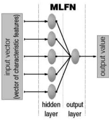
Multilayer feedforward networks (MLFN, also referred to as multilayer perceptrons) are simple but powerful and very flexible tools for function approximation. Figure 3 shows the basic structure of such a MLFN.
and 1), at any other layer the neuron inputs are the outputs of the neurons of the precedent layer. The outputs of every neuron of the last layer are the network outputs. Therefore, it is called output layer. All the others are referred to as hidden layers.
A layer of neurons is determined by its weight matrix, a bias vector and a transfer function. The adjustment of the weight matrix and the bias vector is a matter of the network training, the transfer functions get predifined. Inside a hidden layer a sigmoid transfer function is applied which guarantees, that the layer outputs remain inside the range between−1 and 1. The output layer applies a linear transfer function.
For this application a neural network with one hidden layer was used. In fact, MLFN with a single hidden layer can ap-proximate virtually any function of interest to any degree of accuracy, provided sufficiently many neurons in the hidden layer are available (Hornik et al., 1989). The actual number of hidden neurons has to be estimated by trial and error. The number of neurons in the output layer equals the number of desired outputs.
For further reading on Artificial Neural Networks Hagan et al. (1996) can be recommended.
2.4 Vector of characteristic features
Refering to the previous paragraph, the focus on the setup of the MLFN is the choice of the input vector, i.e. the choice of the relevant features. To keep the problem as simple as possi-ble the output is limited to a single value of flow discharge at a single cross section. (Likewise, this methodology has been applied for stage values too.)
The information relevant for a single target value at a downstream location consists of a finite number of discharge values at the upper boundary locations. The aimin appoint-ing the vector of characteristic features is, in fact, to find all the upstream boundary discharge values that affect the tar-get discharge value at the downstream location. Because of dealing with continuous time series, these discharge values are represented by time steps.
As a first step a sensitivity analysis of a single input value to the output hydrograph has been performed – by applying the hydrodynamic numerical model. The alteration of the discharge value at the timestept0of a single upstream
bound-Fig. 3.Structure of the MLFN.
ary condition influences the output hydrograph between the time stepstminandtmax(Fig. 4).
Ift0stands for time step number zero, the indices min and max represent the numbers of the time steps, between which the alteration of the input value shows an effect at the model output.
Q(input, t0)−> Q(output, tn),min≤n≤max (1)
Q(input, t1)−> Q(output, tn),min+1≤n≤max+1 (2)
. . . (3)
In reverse, assuming that there is only one upstream boundary condition, a single output value at a certain time stept0is only influenced by the input values at the time steps betweent(−max)andt(−min).
Q(input, tn),−max≤n≤−min−> Q(output, t0) (4)
Or:
Q(output, t0)=f (Q(input, tn),−max≤n≤ −min) (5)
That means, that the output value is a function of the in-put values dating back betweentminandtmax(Fig. 5). This methodology has to be applied for every upstream boundary location. The identified input values are the characteristic features for the output values (case 1).
Fig. 4.Sensitivity of the the output hydrograph to a single input value.
Fig. 5.Assignation of time spans to the input vector.
loss in accuracy remains small. The number of characteris-tic features decreases, and certainly the performance will de-cline too. To which extendtforcan be increased, depends on the specific catchment, but certainlytformust not exceed the flow peak propagation time of the main tributaries (case 2).
3 Study area and data
The Mulde catchment (2983 km2)at Erlln gauge, in the Ore mountains (Erzgebirge, East Germany) serves as a first test application of this new methodology. The elevation stretches between some 1200 m and 140 m at the outlet. The land use mainly consists of forest (30%), agricultural land (47%), the remainder being urbanised terrain and fallow. It was heavily affected by the flood of August 2002.
The river reaches in the study area (Fig. 1, Table 1) amount to more than 60 km including parts of the Zschopau and Striegis rivers. 551 cross sections with a mean distance of 120 metres characterise the river bed and the valley. The cross sections are extracted from a digital elevation model (20 m*20 m*0.1 m resolution) combined with data of a ter-restrial survey from the late sixties.
The upper boundary conditions consist of flow hydro-graphs at the inflow gauges, as described in Table 1. As mentioned above, the lower boundary condition must not
in-fluence the target cross section at the Erlln gauge. Therefore, a constant friction slope some 8 km downstream of Erlln was appointed.
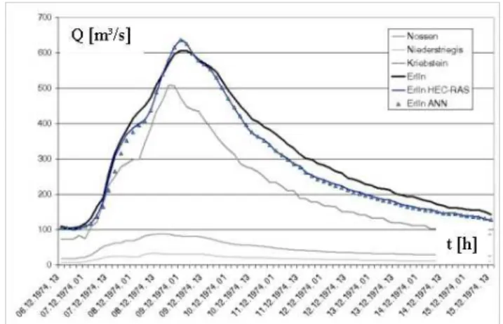
The discharge hydrographs at the upstream boundaries represent about 90 percent of the total area at the outlet. The remaining subcatchments are not equipped with gauging sta-tions. To estimate their influence to the total discharge we applied a rainfall-runoff-model with regionalised parameters. The availability of discharge data with a resolution of one hour is within the scope of expectancy. The mentioned flood of 2002 resulted in a destruction of several gauging stations, amongst them the gauging station at Erlln. The highest stages recorded at every of the four gauges within the study area date back to December 1974. This flood event was used for validation purposes.
4 Results
The flow discharge hydrograph calculated by the hydrody-namic model for the validation flood of 1974 (Fig. 8) shows a good reproduction of the measured one. Rating curves have considerable uncertainties in cases of extreme floods. That is the reason why in these cases absolute values are not very trustworthy. But criteria like the shape and the flood peak propagation time prove to be a good model of the natural system.
The hydrodynamic numerical modelling regarding geo-metrical parameters and the distance between the cross sec-tions requires computation intervals of some 15 seconds. For the generation of the data base of possible extreme flood events time series of 20 years had to be computed.
Table 2.Propagation times to the Erlln gauging station.
Gauge Peak propagation time Influence interval
Kriebstein 6 h 3–9 h
Nossen 8 h 6–9 h
Niederstriegis 6 h 6–7 h
Fig. 6. Characteristic features (blue dots) for the target discharge value (red dot).
target hydrograph (case 1). Reducing this set by the unfilled dots keeps only values within a distance of at least 6 h (min-imum flood peak propagation time) to the target value (case 2).
For both cases MLFN with 15 neurons in the hidden layer were trained. Figure 7 shows a comparison of the network outputs and the outputs of the hydrodynamic model (herein referred to as targets) as normalised values. The mapped data have not been used as training data. In both cases an excellent performance of the trained MLFN can be reported.
Figure 8 compares the output of the MLFN (case 2) with the output of the hydrodynamic model and the measured hy-drograph for the 1974 flood event. The trained MLFN is able to reproduce the performance of the physically based model to a satisfying degree of precision.
Fig. 7.Correlation of MLFN output with output of HEC-RAS, left: case 1, right: case 2).
Fig. 8. Performances of HEC-RAS and the MLFN for the flood event of 1974.
5 Conclusions
This contribution presented a new methodology to com-bine hydrodynamic numerical modelling with artificial intel-ligence. The goal is to overcome both the restricted extrap-olation capabilities of artificial neural networks and the high computation requirements concerning the application of so-phisticated physically based modelling. The advantages of the use of ANN for flood prediction purposes have been em-phasised. Notwithstanding, the ability of a hydrodynamic model to deal with extreme floods beyond recorded events has been incorporated.
Moreover, the hydrodynamic numerical model is an ap-propriate tool to find the characteristic features for the input vector of the MLFN. This is the basis for an efficient utilisa-tion of the input informautilisa-tion.
In fact, the trained MLFN reproduces the model perfor-mance in an excellent manner. The advantages of the use of artificial intelligence are obvious: A noticeable decrease of computation time may be useful for on-line flood forecast-ing. Furthermore, by reducing the vector of characteristic features the forecast horizon can be increased up to the flow peak propagation time.
Edited by: R. Barthel, J. G¨otzinger, G. Hartmann, J. Jagelke, V. Rojanschi, and J. Wolf
Reviewed by: anonymous referees
References
Hagan, M. T., Demuth, H. B., and Beale, M.: Neural Network De-sign, PWS Publishing Company, Boston, 1996.
Hornik, K. M., Stinchcombe, M., and White, H.: Multilayer feed-forward networks are universal approximators, Neural Networks, 2, 5, 359–366, 1989.
Minns, A. W. and Hall, M. J.: Artificial neural networks as rainfall-runoff models, Hydrol. Sci., 41, 399–417, 1996.
Shrestha, R. R., Theobald, S., and Nestmann, F.: Simulation of flood flow in a river system using artificial neural networks, Hy-drol. Earth Syst. Sci., 9(4), 313–321, 2005.
USACE1: US-Army Corps of Engineers, HEC-River Analysis Sys-tem. Hydraulic Reference Manual, Version 3.1, http://www.hec. usace.army.mil/software/hec-ras/, 2002.