Artificial neural networks and linear
discriminant analysis in early selection among
sugarcane families
Luiz Alexandre Peternelli
1*, Édimo Fernando Alves Moreira
1,2,
Moysés Nascimento
1and Cosme Damião Cruz
3Abstract: One of the major challenges in sugarcane breeding programs is an efficient selection of genotypes in the initial phase. The purpose of this study was to compare modelling by artificial neural networks (ANN) and linear discriminant analysis (LDA) as alternatives for the selection of promising sugarcane families based on the indirect traits number of sugarcane stalks (NS), stalk diameter (SD) and stalk height (SH). The analysis focused on two models, a full one with all predictors, and a reduced one, from which the variable SH was excluded. To compare and assess the applied methods, the apparent error rate (AER) and true positive rate (TPR) were used, derived from the confusion matrix. Modeling with ANN and LDA can be used successfully for selection among sugarcane families. The reduced model may be preferable, for having a low AER, high TPR and being easier to obtain in operational terms.
Key words: Plant breeding, artificial intelligence, statistical learning.
Crop Breeding and Applied Biotechnology 17: 299-305, 2017 Brazilian Society of Plant Breeding. Printed in Brazil http://dx.doi.org/10.1590/1984-70332017v17n4a46
ARTICLE
*Corresponding author:
E-mail: peternelli@ufv.br
Received: 19 April 2015 Accepted: 08 September 2016
1 Universidade Federal de Viçosa (UFV), De-partamento de Estatística, Av. PH Rolfs, s/n,
36.570-000, Viçosa, MG, Brazil 2 Instituto Federal do Triângulo Mineiro, Campus Uberaba, 38.064-300, Uberaba, MG, Brazil 3 UFV, Departamento de Biologia Geral INTRODUCTION
Breeding is the basis underlying the entire sugarcane agribusiness. Improved cultivars allow an increase in sugarcane yields as well as enhanced raw material for sugar and alcohol production (Barbosa and Silveira 2012). The most important stage of sugarcane breeding programs is the beginning, called phase T1, when the first genotypes are selected. Thus, selection errors in T1 can foil the success of the entire program (Barbosa and Silveira 2012). In the early stages, selection among families is generally preferred when based on indirect traits (Falconer and Mackay 1996). The indirect traits stalk diameter (SD), number of stalks (NS) and stalk height (SH) are the most commonly used indirect traits to evaluate sugarcane yield and select the best families (Chang and Milligan 1992).
The individual BLUP (Best Linear Unbiased Predictor) (BLUPI) (Resende 2002) and individual simulated BLUP (BLUPIS) (Resende and Barbosa 2006) stand out among the statistical and genetic methods used to select superior materials in many sugarcane breeding programs at T1 stage. It is worth emphasizing that in the case of balanced data, selection by these methods can be simplified. In these cases, it is sufficient to select the families whose mean values exceed the general mean for the target variable real tons of stalks per hectare (TSHr).
TSHr, restricting the selection within the best families in the ratoon phase and the number of families to be evaluated at a time. In other words, because of the time-consuming task, selection using these methods eventually jeopardizes selection in the later stages of the program.
A novel method that is being exploited for different purposes in plant breeding programs, although marginally, is the use of artificial neural networks (Zhou et al. 2011, Barbosa et al. 2011, Barroso et al. 2013, Nascimento et al. 2013, Bhering et al. 2015, Brasileiro et al. 2015, Sant’Anna et al. 2015). This approach is based on principles of statistical learning and artificial intelligence. The basic principle of an artificial neural network is that by providing examples of the relationship between input and output variables, the neural network can be induced to “learn” how to relate these variables (Braga et al. 2000, Haykin 2001). In this way, we can use the variables SD, NS and SH as input variables of the network and the result of the selection process based on TSHr as output variable, in order to select the best families. The great advantage of using neural network modeling is that only a small part of the genotypes would have to be weighted, thus optimizing the selection process.
However, to verify the real efficiency of this technique, it should be compared with the normally applied selection method, based on the variable estimated tons of stalks per hectare (TSHe), as well as on other methodologies, as for example discriminant analysis. Similarly, in linear discriminant analysis we provide samples of traits of two populations or groups to establish a function that is the most discriminating between the populations (Cruz and Carneiro 2006). Thus, we can provide the variables SD, SH and NS of the selected and unselected families based on the selection for TSHr and establish a Fisher’s linear discriminant function to allocate new observations in one of the two groups (selected or unselected families).
The objective of this study was to compare modeling by artificial neural networks with Fisher’s linear discriminant analysis, after simulating and standardizing the input variables, as alternatives for selection among sugarcane families.
MATERIAL AND METHODS
Plant material and phenotypic assessment
The data of five experiments were used, carried out at the Center for Research and Improvement of Sugarcane (CECA), of the Federal University of Viçosa, in the district of Oratórios, Minas Gerais (lat 20° 25’ S; long 42° 48’W, alt 494 m asl). The experiments were arranged in randomized blocks, each with 5 replications and 22 families, totaling 110 families under evaluation. The experimental unit consisted of 20 plants, distributed in two 5-m long rows, spaced 1.4 m apart.
The following traits were evaluated: stalk height (SH) in meters, measuring one stalk per clump, from the base to the first visible dewlap; stalk diameter (SD), in centimeters, measured with a digital caliper at the third internode, counted from the stem base to the apex; total number of stalks per plot (NS) and real tons of stalks per hectare (TSHr), measured by weighing all stalks per plot.
To select the best, the families were weighted in each of the five experiments, and those with a TSHr above the overall experimental mean were selected. In this case, considering normal distribution, the selection rate was 50%. It worth mentioning that any other selection rate could be used, and that in practice the selection rate is lower, according to each breeding program. Here, the idea was only to check whether selection based on classification by ANN and LDA coincides with selection based on TSHr. For the same data set, Moreira and Peternelli (2015) showed that simulation can significantly optimize the performance of a learning technique. In the cited study, the classification technique of linear discriminant analysis was used, and the best results were obtained with 1000 simulated families.
In fact, 110 families is a restricted number to obtain models with generalization capacity, and thus additional values of SD, NS, SH and TSHr were simulated for 1000 families, producing synthetic data, as suggested by Moreira and Peternelli (2015). The values were simulated using the phenotypic mean and covariance structure of each of the five experiments used as training set for a particular scenario, as described below. The simulation was performed using the mvrnorm function of package Mass (Venables and Ripley 2002) implemented in software R (R Development Core Team 2013).
Zi = Vi – V Sd(V)
where:
Zi is the i-th value of the standardized variable;
Vi is the i-th value of the variable to be standardized;
V is the general mean of the variable to be standardized;
Sd(V) is the standard deviation of the variable to be standardized.
Thus, at the end, the data set comprised standardized values of NS, SD, SH, and the result of the selection process via TSHr (Y = 0, if unselected or Y = 1 if selected) for 1110 families in five different scenarios. Each i-th scenario was composed
of 110 original families plus 1000 simulated families as basis for the i-th experiment, i.e., scenario 1 consisted of 110
original families plus 1000 simulated families based on the structure of means and covariances of experiment 1 and so on. In all scenarios, the data set was divided into training and test observations. The training observations are used to adjust the classification rules and the test observations are used to evaluate these rules. In practice, there is no rule separating observations from training and testing. In this study, our interest was to manage to fit a selection model that would circumvent the problem of weighing in the field. To this end, we decided to use only one of the experiments (20% of families) for simulation and training. Thus, in each i-th scenario, the training observations were given by the information
of the 22 families of the i-th experiment plus the information from the 1000 simulated families based on the phenotypic
data of this i-th experiment. The test observations consisted of the 88 families corresponding to the other experiments.
It is important to emphasize that for the application of the learning techniques, the data of NS, SD and SH would have to be collected in all the experiments. The traits NS and SD are relatively simple to assess in the field, whereas the measurement of SH is a rather time-consuming task. Some reasons that complicate SH collection are: great diversity in stalk height within the same family, plant lodging and irregularities in stalk shape.
Thus, to obtain a selection model that would combine selection efficiency and operational simplicity, the analyses were processed with two different models. In model 1, called full, all explanatory variables, i.e., NS, SD and SH, were taken into consideration for fitting. In model 2, called reduced, the variables NS and SD were used, while SH was excluded.
Modelling with artificial neural networks
For modeling using a neural network, two data sets are needed: a training set and a set for network testing. The first is used to adjust the synaptic weights and the second for the evaluation and performance stages of the network. In this study, the training set always corresponds to the experiment underlying the simulation, plus 1000 simulated families. The test set consists of the remaining experiments.
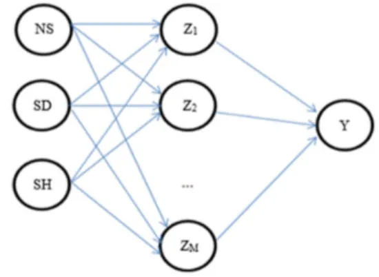
The network used in this study is a multilayer network (Multilayer Perceptron - MLP) with an intermediate layer between the input and the output layer (Hastie et al. 2009), as shown in Figure 1.
Mathematically, NS, SD and SH are the input variables
Zm, where m = 1,2,...,M are functions responsible for the
weighted sum of the inputs. This weighting is done according to the parameters of the network Wi , with i = 1,2,..., I; Y is
the output of the network, i.e., the result of the selection process with the neural network (Hastie et al. 2009).
The activation function used to adjust the synaptic weights was the sigmoid function, given by:
y (x;w) = 1 1+e–wx
The network parameters, or weights, are estimated by
Figure 1. Diagram of an MLP network with an intermediate layer.
minimizing the cross entropy, written as R(θ) = –
N
Σ
i=1 KΣ
k=1 yik logƒk(x i).The minimization is performed by the application of a decreasing gradient algorithm known as back-propagation (Hastie et al. 2009).
The process of network training consists of providing input and output values so that the network “learns” to relate them and thereby estimate the synaptic weights. However, to start the training process initial values for these weights must be provided. According to Venables and Ripley (2002), the initial values can be randomly chosen from a range that satisfies the following equation LS⃰max(|X|)≈1, where LS is the upper limit of the interval and max(|X|) is the highest
module value of the training set.
After the network is trained, it enters the test phase. At this stage, the network was applied to the test dataset and the results were confronted with those obtained by the selection of families with TSHr means exceeding the overall mean.
In the analysis with neural networks we used the nnet function of the nnet package (Venables and Ripley 2002), implemented in R software (R Development Core Team 2013).
Modeling with Fisher’s linear discriminant analysis
The discriminant functions were trained and estimated based on the training dataset, and the efficiency of the method was confirmed based on the respective test set to obtain the apparent error rate. We considered Πi , the groups (selected and unselected families) and μi and Σi, the vector of multivariate means, and the covariance matrix of these
groups with i = 1,2.
The most discriminating linear function between these populations or groups is called Fisher’s Linear Discriminant Function (Ferreira 2011), written as:
D(X) = [μ1– μ2]tΣ–1X.
Taking m = 1
2 [D(μ1) + D(μ2)] as the midpoint between the two univariate population means D(μ1) and D(μ2), the
following classification rule was established:
X ϵ Π1 if D(X) = [μ1– μ2]tΣ–1X > m
X ϵ Π2 if D(X) = [μ1– μ2]tΣ–1X < m.
In practice, it is very difficult to know the mean vectors and covariance matrices. Thus, in most cases the estimators
μi and Σ are necessary (Ferreira 2011).
Thereafter, the parameters μ1, μ2 and Σ will be replaced by the respective estimators X1, X2 and Sc. This will establish Fisher’s Linear Discriminant Sampling Function written as:
D(X) = [x1– x2]tS
c
–1x
Taking m = 1
2 (D(x1) + D(x2)) as the midpoint between the two univariate sample means, a classification rule based
on the samples can be established, which was used to classify the families in selected (Π1) and unselected (Π2), given by:
X ϵ Π1 if D(X) = [x1– x2]tS
c
–1X > m
X ϵ Π2 if D(X) = [x1– x2]tS
c
–1X < m
where X is an observation vector containing the mean NS, SD and SH of the family to be classified.
Discriminant analysis was performed using R software (R development Core Team 2013).
Evaluation and comparison of methods
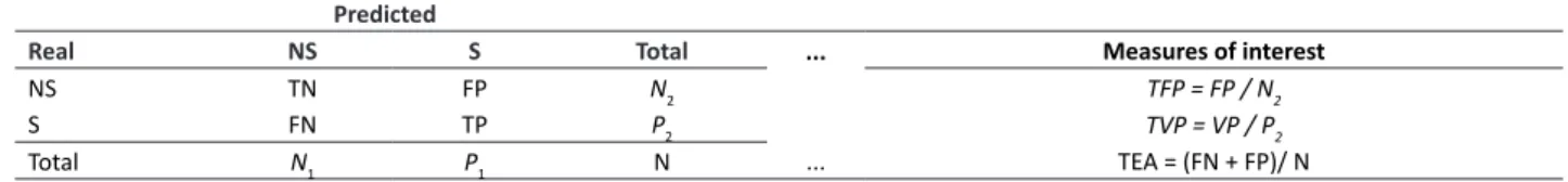
the variable TSHr versus the number of classifications predicted by the classifier considered for each class based on the test set. A general scheme for the confusion matrix is shown in Table 1.
Several measures can be derived from the confusion matrix for the evaluation of the classifier. Specifically with regard to the selection of sugarcane families, we are interested in the apparent error rate (AER), which indicates the number of families classified incorrectly by the classification method considered. Another measure of interest is the true positive rate (TPR), which shows the percentage of correctly selected families by the studied classification method.
RESULTS AND DISCUSSION
As pointed out, the values for apparent error rate (AER) are low by both classifiers, the neural network (ANN) and discriminant analysis (LDA), when the full model (model 1) is used. For the classifier ANN, the mean AER was 0.0977, and 0.1366 for LDA. It is worth highlighting that a mean AER of 0.0977 indicates that on average only 09.77% of the families were misclassified. Although the absolute value of the mean AER of the classifiers suggests that ANN performs better than LDA, it should be emphasized that the confidence intervals constructed for the mean AER of these classifiers suggest that they are equal for the full model (Table 2, Figure 2).
With respect to the true positive rate (TPR), the two classifiers ANN and LDA also have a satisfactory performance when using the full model. The mean TPRs for the ANN and LDA models were 0.9378 and 0.8962, respectively. It is important to highlight that a TPR of 0.9378 indicates that the classifier under study also selected 93.78% of the families selected by the method considered ideal. As with the mean AER, the confidence intervals for the mean TPR of the classifiers suggest that the classifiers are statistically equal when the full model is used (Table 2, Figure 3).
For the reduced model, the classifiers ANN and LDA also had low AER values in all scenarios. In other words, the probability of a selection error by the classifiers is low in all scenarios. In this model, the mean AERs for the classifiers ANN and LDA were, respectively, 0.0954 and 0.1068. The confidence interval constructed for the mean of these classifiers indicates that they can be considered equal in the reduced model (Table 2, Figure 2).
Moreover, for the reduced model, the TPR was also high in all scenarios for both classifiers. This indicates that the classifier in use will also select most of the families selected by the method considered ideal. The mean TPRs in the Table 1. General diagram of a confusion matrix (right) accompanied by some measures of interest derived from it (left)
Predicted
Real NS S Total ... Measures of interest
NS TN FP N2 TFP = FP / N2
S FN TP P2 TVP = VP / P2
Total N1 P1 N ... TEA = (FN + FP)/ N
*NS = Not Selected; S = Selected; TN = True Negative; FP = False Positive; FN = False negative; TP = True Positive; AER = Apparent Error Rate; TPR = True Positive Rate and FPR = False Positive Rate. Real indicates selection by the method considered ideal (real tons of sugarcane per hectare) and Predicted shows selection with an alternative classification method (artificial neural network and linear discriminant analysis).
Table 2. Apparent error rate (AER) and true positive rate (TPR) for artificial neural networks (ANN) and linear discriminant analysis
(LDA) in five different scenarios in two models: model 1 (full, with all predictors) and 2 (reduced, without the predictor stalk height) Scenario
Method Model 1 2 3 4 5 Mean CI 95%
AER ANN 1 0.0795 0.0909 0.1136 0.1250 0.0795 0.0977 [0.0721; 0.1233]
2 0.1022 0.0795 0.1136 0.1023 0.0795 0.0954 [0.0765; 0.1144]
LDA 1 0.1250 0.1250 0.1591 0.1477 0.1363 0.1386 [0.1202; 0.1570]
2 0.1136 0.0909 0.1250 0.0909 0.1136 0.1068 [0.0879; 0.1257]
TPR ANN 1 0.9574 0.9184 0.9184 0.9375 0.9574 0.9378 [0.9136; 0.9620]
2 0.9167 0.9184 0.8979 0.9583 0.9362 0.9255 [0.8972; 0.9538]
LDA 1 0.9149 0.8979 0.8367 0.9167 0.9149 0.8962 [0.8538; 0.9386]
reduced model were 0.9255 and 0.8999, respectively, for the ANN and LDA classifiers. Note the closeness of the mean values, and in fact, the confidence interval for the mean of these classifiers suggests that they can be considered equal (Table 2, Figure 3).
Importantly, the exclusion of the SH variable from the set of explanatory variables did not lead to a significant performance loss of the classifiers. In other words, the results for AER and TPR in both classifiers were similar for both models (Table 2). The resulting confidence intervals suggested equality between the full and reduced models in all possible situations (Figures 3 and 4).
The low AER and high TPR values obtained by both classifiers and both models shows that ANN and LDA could be used successfully in the selection of sugarcane families. However, due to the greater ease of operation of the reduced model, it may be preferred. The great advantage of using this strategy for selection of sugarcane families is that it would be necessary to weigh only a small part of the genotypes. In this study, by weighing only one of five experiments (training experiment) there was an excellent generalization for the remaining four experiments (test experiments). Thus, it is evident that this strategy could considerably reduce the fieldwork, optimizing the selection process.
Of course, for the selection of the best families, NS and SD would have to be determined for all families. However, we assumed collecting these data would be simpler than the weighting of all the experimental plots. Differently from the results obtained in this study, in a diversity study of papaya (Carica papaya L) accessions of Barbosa et al. (2011), and in a study with simulated genotypic data of 10 populations in Hardy-Weinberg equilibrium by Sant’Anna (2015), the authors concluded that as classifier, the neural network is superior to conventional discriminant analysis.
In fact, Haykin (2001) reported that neural network models are more flexible and thus normally able to describe more general relationships in data than traditional models. On the other hand, linear discriminant analysis is only fully functional for linearly separable problems (James et al. 2013). Thus, the good results for discriminant analysis, the low apparent error rate and high true positive rate in this study indicate that the problem in question is linearly separable.
Despite the good results obtained with these classifiers, it is worth mentioning that other classification techniques can be applied. Among these, we can mention the classifiers k-nearest neighbors, support vector machines and decision trees, among others techniques.
CONCLUSION
Figure 2. Mean apparent error rate (AER) and confidence
inter-val for the classifiers, artificial neural network (ANN) and linear discriminant analysis (LDA), in two models, full (with all predic-tors) and reduced (exclusion of the variable stalk height from the predictor set).
Figure 3. Mean true positive rate (TPR) and confidence interval
Selection based on modeling with artificial neural networks or linear discriminant analysis shows high agreement with selection by TSHr and can be successfully used for selection among sugarcane families. The reduced model, which was adjusted according to the traits NS and SD, may be preferred over the full model, adjusted according to the traits NS, SD and SH, due to the greater ease of data collection in the field.
ACKNOWLEDGEMENTS
The authors thank the Inter-University Network for the Development of Sugarcane Industry (RIDESA) for providing the data and for the constant financial support for the breeding program development, and CAPES, CNPq and FAPEMIG for the financial support for research projects.
REFERENCES
Barbosa CD, Viana AP, Quintal SSR and Pereira MG (2011) Artificial neural network analysis of genetic diversity in Carica papaya L. Crop Breeding and Applied Biotechnology 11: 224-231.
Barbosa MHP and Silveira LCI (2012) Melhoramento genético e recomendação de cultivares. In Santos F, Borém A and Caldas C (eds) Cana-de-açúcar, bioenergia, açúcar e etanol – tecnologias e
perspectivas. Folha de Viçosa, Viçosa, p. 313-331.
Barroso LMA, Nascimento M, Nascimento ACC Silva FF and Ferreira ARP (2013) Uso do método de Eberhart e Russel como informação a priori para aplicação de redes neurais artificiais e análise discriminante visando à classificação de genótipos de alfafa quanto à adaptabilidade e estabilidade fenotípica. Revista Brasileira de Biometria31: 176-188. Bhering LL, Cruz CD, Peixoto LA, Rosado AM, Laviola BG and Nascimento M (2015) Application of neural networks to predict volume in eucalyptus. Crop Breeding and Applied Biotechnology 15: 125-131. Braga AP, Carvalho ACPLF and Ludermir TB (2000)Redes neurais
artificiais: teoria e aplicações. LTC – Livros Técnicos e Científicos, Rio de Janeiro, 262p.
Brasileiro BP, Marinho CD, Costa PMA, Cruz CD, Peternelli LA and Barbosa MHP (2015) Selection in sugarcane families with artificial neural networks. Crop Breeding and Applied Biotechnology 15: 72-78. Chang YS and Milligan SB (1992) Estimating the potential of sugarcane
families to produce elite genotypes using univariate cross prediction methods. Theoretical and Applied Genetics84: 662-671.
Cruz CD and Carneiro PCS (2006) Modelos biométricos aplicados ao
melhoramento genético. Editora UFV, Viçosa, 585p.
Falconer DS and Machay TFC (1996) Introduction to quantitative genetics. Longmans Green, Malaysia, 463p.
Ferreira DF (2011) Estatística multivariada. Editora da UFLA, Lavras, 675p. Hastie T, Tibshirani R and Friedman J (2009) The elements of statistical
learning: data mining, inference, and prediction. Springer, New York, 745p.
Haykin S (2001) Redes neurais princípios e prática. Bookman, Porto Alegre, 900p.
James G, Witten D, Hastie T and Tibshirani R (2013) An introduction to statistical learning: with applications in R. Springer, New York, 426p. Moreira EFA and Peternelli LA (2015) Sugarcane families selection in early stages based on classification by linear discriminant analysis. Revista Brasileira de Biometria33: 484-493.
Nascimento M, Peternelli LA, Cruz CD, Nascimento ACC, Ferreira RP, Bhering LL and Salgado CC (2013) Artificial neural networks for adaptability and stability evaluation in alfalfa genotypes. Crop Breeding and Applied Biotechnology 13: 152-156.
R Development Core Team R (2013) A language and environment for statistical computing. R Foundation for Statistical Computing, Vienna. Avaliable at <http://www.r-project.org>. Accessed in November 2013. Resende MDV (2002) Genética biométrica e estatística no melhoramento
de plantas perenes. Embrapa Informação Tecnológica, Brasília, 975p.
Resende MDV and Barbosa MHP (2006) Selection via simulated Blup based on family genotypic effects in sugarcane. Pesquisa Agropecuária
Brasileira 41: 421-429.
Sant’Anna IC, Tomaz RS, Silva GN, Nascimento M, Bhering LL and Cruz CD (2015) Superiority of artificial neural networks for a genetic classification procedure. Genetic and Molecular Research 14: 9898-9906.
Venables WN and Ripley BD (2002) Modern applied statistics with S. Springer, New York, 493p.