AT-SITE FLOOD ANALYSIS USING
EXPONENTIAL AND GENERALIZED
LOGISTIC MODELS IN PARTIAL
DURATION SERIES (PDS)
M.K.Bhuyan1, Joygopal Jena2, P.K. Bhunya3
1Research Scholar,
Siksha O Anusandhan (SOA) University, Bhubaneswar, Odisha, India- 751030.
2 Professor,
Gandhi Institute of Technogical Advancement, Bhubaneswar, Odisha, India- 752054
3 Associate Professor,
Kalinga Institute of Industrial Techonolgy, Bhubaneswar, Odisha, India-751024
1[email protected] 2[email protected] 3[email protected]
Abstract - Flood Frequency Analysis (FFA) uses both flood peak series, i.e. Annual Maximum Series (AMS) and Partial Duration Series (PDS). AMS analyses number of peaks equal to number of observation years using a single best fit probability distribution, while PDS analyses peaks over a threshold value adopting Poisson distribution (PD) and negative binomial (NB) distribution counting occurrences of peaks (μ) over threshold and exponential distribution (ED), generalized logistic distribution (GLD) or Pareto distribution (GP) for magnitude. Both ED and GLD method are used to analyze at-site extreme flood information in the PDS model at Champua gauging site under Baitarani Basin, Odisha (India). Performances of AMS/PD-ED, AMS/NB-ED, AMS/PD-GLD, AMS/NB-GLD are compared in terms of uncertainty of T-year event estimator. Results show AMS/PD-ED model yields lower variance of T-year estimate than AMS/NB-ED model, while AMS/NB-GLD gives less variance in comparison to AMS/PD-GLD. Results indicate that in case of ED, flood quintiles are acceptable for μ≤8 and T≤500 within 95% confidence limit, while they are comparable for μ≤3 and T≤100 in case of GLD distribution. To summarize, NB distribution is preferred for number of flood peaks if coupled with GLD for flood exceedances and Poisson distribution in case of ED for flood exceedances values.
Keywords -Annual Maximum Series, Partial Duration Series, Exponential Distribution, Generalized Logistic
Distribution
I. INTRODUCTION
of AMS. The AMS sample is usually rather small as compared to PDS sample where more than one flood per year may be included. PDS models are used for flood frequency analysis (FFA) where the flood record is short. If the threshold is increased to certain limit, recurrence interval of large events computed using AMS and PDS models tend to converge. Since the PDS sample is defined by all peaks that lie above a certain truncationlevel, assuring the independence of data series and choosing an appropriate threshold value is of prime importance.
The methods followed for formulating these models are quite different e.g. an AMS model uses a cumulative distribution function (cdf) to model the flood extremes, whereas the PDS model uses two probabilistic models: (a) one for the probability of occurrence of peaks above a threshold, and (b) the cdf, ˜˜ for
modeling the flood exceedance. Generally more than one distribution may fit the data well and selecting the best model can be difficult (Salas et al.2012). Different countries have formulated guidelines regarding use of various distributions. Further the behavior of the method also depends on the estimation technique for distribution parameters which are estimated through different methods such as methods of moments (MOM), methods of probability weighted moments(PWM)/L-moments and maximum likelihood estimation (MLE). The present study is focused on at-site flood analysis using the PDS model for quantile estimation using the L-moment method with two probability distribution function, i.e. ED and GLD. The numbers of exceedances are modeled as a discrete distribution whereas the exceedances magnitudes are modeled as continuous distribution and their total probability leads to flood magnitude of desired return period (QT). Considering the number of
flood peaks above the threshold (Q0) as random, Shane and Lynn (1964) assumed this number to follow a PD.
Since the process following a PD assumes that events are independent and occur uniformly throughout the interval of observations, it necessitates that there is no clustering of events (Stark and Woods, 1986). Thus, the dependence of flood peaks in PDS may well have an effect on the ability of PD to describe the number of peaks above threshold. Besides PD (Todorovic & Zelenhasic 1970[29], NERC 1975[21], Cunnane 1979[5], Lang
et al.
1997[16], ÖnÖz and Bayazit2001 [23], Bhunya et al. 2012[2]), Negative Binomial (NB) ( Cunnane 1979[5], Lang et
al. 1997[16], ÖnÖz and Bayazit2001[23] , Bhunya et al. 2012[2]) and Binomial (Lang et al. 1997[16], ÖnÖz and
Bayazit2001[23]) can also be chosen. Studies by NERC (1975) [21,22] and Cunnane (1979) [5] on 26 streams in
Great Britain indicated that the number of peaks occurring each year is not a Poisson variate since its variance was significantly greater than its mean, which violates the basic assumption of PD. As NB distribution has this property, it was used by Lang. (1999) [15] and ÖnÖz and Bayazit(2001) [23] in PDS modeling.
Many commonly used distributions are approximately exponential with a stretched upper tail, for which ED was first used by Kirby (1969) [13] to fit the flood exceedances in a PDS model. Although alternate
frequency distributions have been proposed in the past, e.g. the Gamma distribution (Zelenhasic 1970[30]),
Weibull distribution (Ekanayake and Cruise 1993[7]), Generalized logistic model (Bhunya et al. 2012[2]) in PDS
models, and the most popular is the generalized Pareto (GP) distribution which has the ED as a special case (Fitzgerald 1989[8]; Madsen
et al. 1997[18]; Martins and Stedinger 2000[19], 2001[20]; Bhunya et al. 2013[3]). All
these studies use GP distribution as the flood exceedance model with PD arrival rate for deriving the PDS model. Recently ÖnÖz and Bayazit(2001) [23]compared the advantages of NB and Poisson distributions in PDS
model when ED is used as the flood exceedances model. Bhunya et al. (2012[2], 2013[3]) found that the Poisson
distribution is better than the NB distribution in cases where the mean and variance of the annual number of exceedances are small. However, their studies stressed the importance of threshold selection as main criteria for the performance of the PDS models rather than the choice of any particular distribution to model the arrival rates.
With the above background, the present study compares the merits of PD and the NB distribution as models for the occurrences of peaks exceeding a threshold in PDS context, considering ED and GLD to model the flood exceedances. Estimation of the ED and GLD parameters by the method of L-moments (Greenwood et al. 1979[9]; Hosking 1986[10]; Hosking & Wallis 1997[11], Shabri & Jemain 2013[27]) is formulated for different
thresholds. The performances of the AMS/PD-GLD and GLD and also AMS/PD-ED and AMS/NB-ED models are compared using the variances of T-year estimates on field data. These are also compared with the corresponding AMS analysis considering the maximum annual peak values matching to the period of data available.
II. PROBABILITY DISTRIBUTIONS USED IN ANALYSIS
A. Exponential Distribution
The exponential distribution is a special case of the Gamma family of distributions (Rao & Hamed 2000[24]) and
( )
( )∞
≤
≤
ξ
−
=
β ξ − −Q
,
e
1
Q
F
Q (1)ξ
is the lower bound and β is the scale parameter.Eqn.1 in the inverse form is expressed as
( )
(
)
β
−
ξ
=
−
β
−
ξ
=
T
1
ln
Q
F
1
ln
Q
T (2)The parameters
ξ
and β in terms of L-moments are given as2 1
−
β
and
β
=
2
λ
λ
=
ξ
(3)( )
=
β
+
T+
T2
2T
N
1
2
K
3
4
K
Q
Var
, whereK
T=
ln
( )
T
−
1
(3i)KT is the growth factor for exponential distribution.
B. Generalized Logistic Distribution
The probability distribution function of a three parameter generalized logistic distribution is defined by Hosking and Wallis (1997) as
( )
(
)
(
)
,
k
0
0
k
,
Q
Q
k
1
ln
k
1
Q
F
=
≠
α
ξ
−
α
ξ
−
−
−
=
(4)k
,
,
α
ξ
are the location, scale and shape parameters, respectively. The T year event QT is defined as(
)
(
k)
(
(
)
k)
TT
k
1
T
1
1
k
1
T
1
K
Q
=
ξ
−
−
ξ
α
+
ξ
=
−
−
α
+
ξ
=
− − (5)KT is the growth factor for GLD. The location parameter
ξ
is equated to the distribution median to the samplemedian m (
ξ
= m ).(6)
with m=
λ
1 and α=λ
2 when expressed in L-moment estimators.Ahmad et al. (1988) [1], Hosking and Wallis (1997) [11], Rao and Hamed (2000) [24] expressed the general form of
the distribution to be used in flood exceedances model
(
Q
Q
0)
m
1exp
1
)
Q
(
F
−
α
−
−
−
+
=
(7)and the flood quantile is expressed as
Q
T=
Q
0+
m
+
α
ln
(
T
−
1
)
(8) C. Poisson DistributionIn the PDS model, all peak events above a threshold level are considered and the number of these peaks in a given year is assumed to follow a Poisson distribution having the probability mass function:
r!
N)
(
e
r)
P(X
=
=
μNµ
r−
r= 0, 1, 2 … (9)
where P(X= r) is the probability of r events in N years, μ is the average number of threshold exceedances. Eqn.(9) is true as long as the flood peaks are independent (Langbein 1949[17]). For n number of observed
(
)
(
2)
T 2
T N 3 2.3361K
Q
exceedances in N years, μ is equal to n/N. For Poisson distribution, PWM estimations and the population estimate of μ is given by
N
n
μˆ
=
(10)The mean and variance of r are defined as follows:
2
σ
Var(r)
n/N
μ
E(r)
=
=
=
=
; n ≥ 5 (11)For μ > 5 the distribution of r is symmetrical and it asymptotically approaches a normal distribution (Johnson and Kotz 1973[12]). For no flood exceedances to occur in a given year, substituting r = 0 in Eq. (1), the
following is obtained
μ 0 μ
e
0!
)
(
e
0)
P(r
=
=
−µ
=
− (12)which is the probability distribution function (pdf) of an exponential distribution. The cumulative mass function of Eq. (9) for N years is given by
( )
X
1
μe
μNF
=
−
− ; N > 0 (13)where X is a variate. Assume that a threshold level Q0 is chosen, corresponding to a mean annual number of
exceedances of Poisson distribution μ ; then at any higher threshold Q > Q0, the number of exceedances
r
′
isPoisson distributed with the following parameter (Flood Studies Report 1975)
[
1
F(Q)
]
μ
μ
′
=
−
(14)Since F (Q) ≤ 1, it follows that
μ
′
≤
μ
i.e. the truncated mean of exceedances above the new threshold q decreases, which is quite obvious.D. Negative Binomial Distribution
Binomial random variable is a count of number of successes in certain number of trials, whereas the negative binomial distributed variables are literally opposite to that; here the number of successes are predetermined and the number of trial are random. The NB distribution is the probability of having to wait X(= r+k-1) trials to obtain r-1 successes and the success in r+k trial. If X has a NB distribution with parameters p and r , the probability mass function is given by,
( )
r k 1 r k 1
-r
p
(1
p)
r)
P(x
=
=
+ −−
; r > 1 and 0 ≤ p ≤ 1 (15)In Eq.(15) p is the constant probability of a success in any independent trial . P(X=r) gives the probability that the variate X is equal to r. Because at least r trials are required to get a success, the range of Eq.(7) is from r to ∞. The probability that there is no flood exceedance in any given year is obtained by making r-1 = 0 in Eq. (15) as
( )
k 1 k k0
(1
p)
(1
p)
0)
1
-P(r
=
=
−−
=
−
(16)Similarly, the probability of number of occurrences of exceedances less than r is given by
(
)
r kr
0 r
1 k r
r
p
(1
p)
r]
P[x
≤
=
−
= − +
(17) The value of p and r are given by (Spigel 1987) as
(
)
(
)
(
)
(
0)
0 0
r
1
p
p
and
p
V
E
Q
Q
-
-
Q
Q
Q
Q
E
−
=
µ
=
−
=
(18)III. PDS BASED ANNUAL MAXIMUM FLOODS
The annual maximum flood in the PDS model is determined from the total probability of average number of flood exceedances and the exceedances value above the threshold. The probability distribution function F(Q) is given by (Shane and Lynn 1964)
( )
∞( ) ( )
(
)
=µ
=
0 r
r
y
G
r
P
Q
F
where y= Q-QoA. AMS/PD-ED Model
When number of exceedances are poissonian and their magnitudes are exponential (AMS/PD-ED) (Zelenhasic 1970[30]; ÖnÖz and Bayazit 2001[23])
( )
∞ = µ
β
−
−
µ
−
=
β
−
−
µ
=
0 r 0 rr
1
exp
y
exp
exp
Q
Q
e
Q
F
(20)β is the single parameter of exponential distribution = E(y) = μ = Var(y)0.5
Eq.(20) is the Gumbel or EV1 distribution widely used in FFA. On simplification of Eq.(20) with
( )
T
1
1
Q
F
=
−
, T being the return period, we getT 0
T
Q
ln
Y
Q
=
+
β
µ
+
β
(21)where
−
−
−
=
T
1
1
ln
ln
Y
T is the Gumbel reduced variate.Cunnane (1973) [4] obtained the following expression for the asymptotic sampling variance of the estimate Q T
computed from N-year long observations:
( )
{
[
]
2}
T 2
T
N
1
ln
Y
Q
Var
+
µ
+
µ
β
=
(22)Rosberg (1985) introduced a small sample correction factor to the above formula which is of minor importance for μN> 10.
B. AMS/NB-ED Model
When number of exceedances are negative binomial and their magnitudes are exponential (AMS/NB-ED) (ÖnÖz and Bayazit 2001[23])
( )
∞(
)
(
)
=
β
−
−
−
−
−
=
β
−
−
−
−
−
+
=
1 r k k r kr
1
p
1
exp
y
1
p
1
p
1
exp
Q
Qo
p
1
r
1
k
r
Q
F
(23) which gives
−
−
β
−
−
β
+
=
−1
T
1
1
ln
p
1
p
ln
Q
Q
r 1 0T (24)
And the variance is given as
(25)
C. AMS/PD-GLD Model
When number of exceedances are poissionian and their magnitudes are GLD distributed (AMS/PD-GLD) (Bhunya et al. 2012[2])
( )
∞( )
[
( )
]
= − µ −
α
µ
α
+
−
−
−
−
=
α
−
−
−
+
µ
=
0 r r 1r
Q
Qo
m
ln
exp
exp
m
Qo
Q
exp
1
!r
e
Q
F
(26)Eq.(26) reduces to
( )
T0
T
Q
ln
m
Y
Q
=
+
α
µ
+
+
α
(27)The variance is given by
(28)
D. AMS/NB-GLD Model
When number of exceedances are negative binomial and their magnitudes are GLD distributed (AMS/NB-GLD) (Bhunya et al. 2012[2])
( )
( ) (
)
r 1 0 k r 1 kr
1
p
1
exp
Q
Qo
m
1
exp
Q
Qo
m
p
1
r
1
k
r
Q
F
α
−
−
−
+
=
α
−
−
−
+
−
−
−
+
=
− ∞ = −
(29)Eqn.(29) gives the flood of a given return period as follows
(30) The variance is given by
(31)
IV. STUDY AREA
The gauging station at Champua on River Baitarani (Fig.1) is selected for the present study. River Baitarani up to this gauging site records the river hourly gauge values and the discharges at 8.00 AM everyday and the records are available for the period 1991 to 2013 (23 years). The hourly discharges are computed from the Gauge Discharge curve prepared using the recorded daily gauge and discharge values during the monsoon period. For the PDS model, the maximum daily maximum discharge values are used for analysis, whereas the yearly maximum values are considered for AMS analysis. Table.1 provides the discharge statistic of River Baitarani at Champua.
TABLE 1 Flow parameters of the GD site
Period Annual. Discharge (m3/s) Mean(μ) (m3/s) SD(σ) (m3/s) Skewness (ϒ) Maximum Minimum
1991-2013 2756.38 156.79 919.90 612.04 1.19
( )
(
)
+
+
µ
+
µ
α
=
1
0
.
7107
ln
Y
3
N
Q
Var
2 T 2 T( )
−
−
α
−
+
=
−1
T
1
1
ln
m
Q
T
Q
r 1 0(
)
(
( )
)
( )
( )
(
)
(
)
(
)
( )
(
)
[
− −]
α Fig 1 Index map of Baitarani Basin (GD site at Champua) V. RESULTS AND DISCUSSION
The performance of exponential (ED) and generalized logisticdistribution (GLD) are compared on the basis of their variance ratio defined as
( )
( )
TT**//GLDEDi
Var
Q
Q
Var
R
=
i = 1 to 4 as defined in Table.6 (* is PD/NB)If the value of Ri for a given period is greater than one, it indicates that GLD yields less variance than the ED
when used for fitting the flood exceedances in PDS and the value equal to one is the ideal. The results with respect to the data used for AMS/PD-ED, AMS/NB-ED, AMS/PD-GLD and AMS/NB-GLD analysis are given in Tables. 2-5.
As indicated in Table.6, the variance ratio R1 indicates that AMS/PD-ED yields lesser variance than
AMS/NB-ED for all mean number of exceedances except for μ=2, σ2=4.727 for T=5 to 500. Earlier Cunnane (1979) [5] has
found that there is no satisfactory improvement by employing binomial distribution instead of Poisson distribution to account for flood exceedances in PDS. In a similar study ÖnÖz and Bayazit (2001) [23] also
concluded that flood estimates based on NB distribution is almost identical to those obtained using Poisson distribution. They used Var(QT) as an index to compare the AMS/PD-ED and AMS/NB-ED model. Similarly in
case of GLD, AMS/PD-GLD gives more variance compared to AMS/NB-GLD except for μ=1.478, σ2=2.351.
The R3 values further indicate that the variance ofAMS/PD-ED model is smaller than AMS/PD-GLD model
when the μ ≥4.The R4 values indicate the AMS/NB-ED always generates excess variance than AMS/NB-GLD model for μ≤6. But since it is seen that when μ ≤ 3, the POT and AMS model agrees with each other to a greater extent. In the present at-site analysis, the findings are also in agreement with that of Cunnane (1979) [5]
and ÖnÖz and Bayazit(2001) [23]. When the value of number of exceedances (μ) is in between 1.478 to 3, the
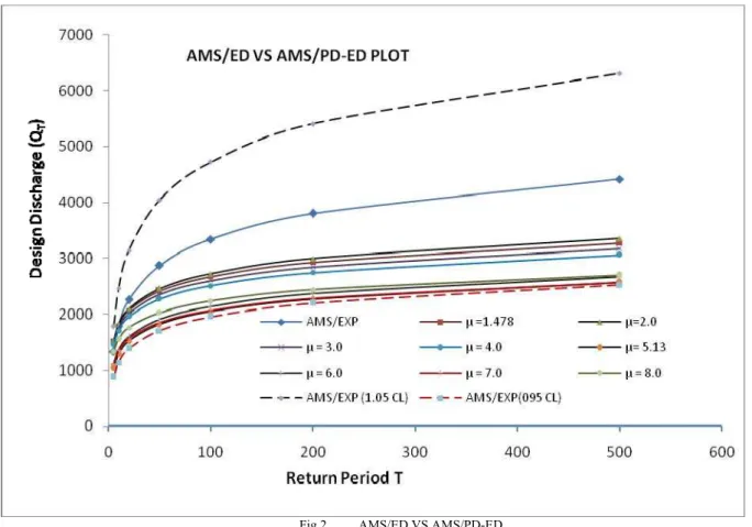
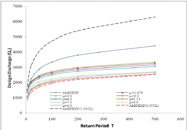
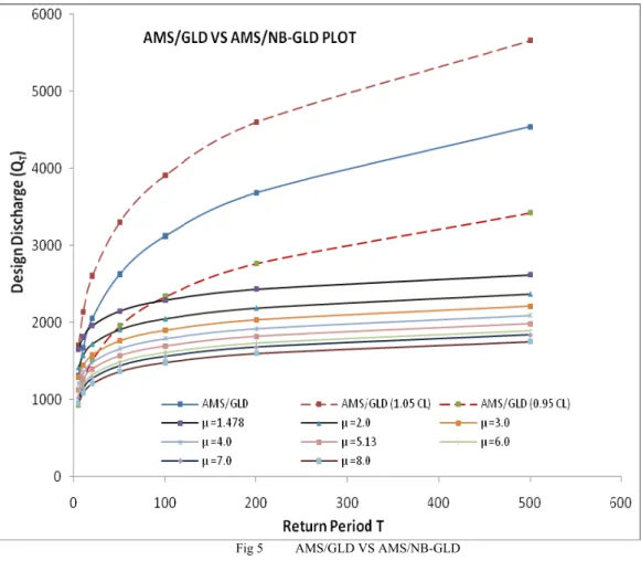
standard deviation (σ) is nearly equal to the value of μ which is the basic property of a Poisson distribution. The variance ratio justifies that AMS/PD-ED model performs better than the AMS/PD-GLD model. In case GLD is to be used, AMS/NB-GLD is preferable to AMS/PD-GLD. In the entire analysis it is seen that PDS based AMS model results are more than the AMS model for μ=1.478, σ2=2.351. Figure 2-5 give a better visual match
in case of ED the flood quintiles are quite acceptable for μ≤8 and T≤500 within 95% confidence limit, while they are comparable for μ≤3 and T≤100 in case of GLD distribution.
Fig 3 AMS/ED VS AMS/NB-ED
Fig 5 AMS/GLD VS AMS/NB-GLD
VI. CONCLUSION
The analysis presented here focused on the choice between exponential distribution and the generalized logistic distribution both in the AMS and PDS model. In the AMS model the flood quantiles are computed using the annual maximum observed floods and in PDS model using the flood exceedances above a threshold coupled with Poisson and negative binomial distribution for mean number of flood exceedances. The variances of the flood quantile estimates are compared through R1 to R4 values in order to determine the superiority of the
distributions employed in the study in the PDS format and also compared with the AMS model. The choice of the most efficient T-year event estimator model is not only dependent on whether it is AMS or PDS, but also the method of parameter estimation of the probability distributions used. Here in the present case only L-moment method of parameter estimation has been followed. It is seen that these ratios are not dependent on the years of data available but is a function of the mean and variance and the distribution parameters. The difference between the estimations under AMS and PDS model becomes prominent with increase in T years and with increase in value of μ. A good match between the quantile values in PDS has been noticed so long the value of μ is less than 3. The values of the ratio of Var(QT) as given in Table.3 infers that AMS/NB-GLD gives less
variance of the QT comparedto AMS/NB-ED for the field data of Champua gauging site under Baitarani basin.
This is in quite agreement to the finding of Bhunya et al. (2012) [2] who used data of a different region. Similarly
in case of flood exceedances of exponential distribution, AMS/PD-ED model performs better than the AMS/NB-ED model for the present field data. The advantage of Poisson distribution over negative binomial distribution has been studied by ÖnÖz and Bayazit(2001) [23]. He has reported that the flood estimates and their
corresponding variance based on negative binomial distribution when combined with ED for the flood exceedances are almost identical to those obtained using PD. The present finding is also in agreement with ÖnÖz and Bayazit(2001) [23], so also Kirby (1969) [13] and Cunnane (1979) [5]. To summarize the NB distribution
should be preferred for number of flood peaks if to be coupled with GLD for flood exceedances and Poisson distribution in case of ED for flood exceedances values.
TABLE.2
Design Discharge (QT) and Var (QT) for AMS/PD-ED
μ= 1.478 2.000 3.000 4.000 5.130 6.000 7.000 8.000
var= 2.351 4.727 8.273 12.091 17.027 22.727 27.545 37.545
Qo = 805.097 677.600 553.700 469.446 400.648 344.554 313.350 294.884
T QT Var(QT) QT Var(QT) QT Var(QT) QT Var(QT) QT Var(QT) QT Var(QT) QT Var(QT) QT Var(QT)
5 1512.57 18842.90 1525.92 18897.25 1485.36 14442.68 1452.28 11760.09 1036.71 9708.87 1109.92 9355.58 1101.54 7767.75 1332.97 6313.78 10 1793.38 32850.84 1816.20 31435.43 1754.42 22757.50 1707.82 17929.77 1280.79 14432.51 1357.77 13706.00 1335.43 11228.01 1550.61 9026.93 20 2062.74 50647.00 2094.64 46904.83 2012.50 32704.92 1952.94 25181.80 1514.92 19912.45 1595.52 18715.61 1559.79 15185.74 1759.37 12113.24 50 2411.40 80020.99 2455.05 71933.84 2346.56 48447.65 2270.23 36508.38 1817.97 28385.40 1903.26 26416.48 1850.19 21237.11 2029.59 16811.58 100 2672.67 106720.45 2725.13 94391.35 2596.89 62364.78 2507.99 46430.48 2045.07 35755.06 2133.86 33086.80 2067.81 26458.43 2232.09 20852.57 200 2932.99 137316.67 2994.22 119921.00 2846.31 78037.60 2744.88 57538.55 2271.33 43967.23 2363.63 40499.28 2284.63 32245.77 2433.84 25322.06 500 3276.43 183782.28 3349.24 158419.26 3175.37 101473.64 3057.41 74059.99 2569.85 56129.35 2666.76 51449.21 2570.69 40774.55 2700.02 31895.63
TABLE. 3
Design Discharge (QT) and Var (QT) for AMS/NB-ED
μ= 1.478 2.000 3.000 4.000 5.130 6.000 7.000 8.000
var= 2.351 4.727 8.273 12.091 17.027 22.727 27.545 37.545
Qo = 805.097 677.600 553.700 469.446 400.648 344.554 313.350 294.884
T QT Var(QT) QT Var(QT) QT Var(QT) QT Var(QT) QT Var(QT) QT Var(QT) QT Var(QT) QT Var(QT)
TABLE.4
Design Discharge (QT) and Var (QT) for AMS/PD-GLD
TABLE.5
Design Discharge (QT) and Var (QT) for AMS/NB-GLD
μ= 1.478 2.000 3.000 4.000 5.130 6.000 7.000 8.000
var= 2.351 4.727 8.273 12.091 17.027 22.727 27.545 37.545
Qo = 805.097 677.600 553.700 469.446 400.648 344.554 313.350 294.884
T QT Var(QT) QT Var(QT) QT Var(QT) QT Var(QT) QT Var(QT) QT Var(QT) QT Var(QT) QT Var(QT) 5 1657.74 12246.48 1421.63 8048.19 1290.86 8980.19 1205.55 9312.80 1128.72 9258.81 1063.05 8685.10 1023.81 8807.80 955.23 7876.61 10 1813.89 17622.85 1578.15 12336.36 1441.94 13238.75 1350.88 13520.75 1268.32 13334.45 1199.48 12532.47 1156.97 12635.41 1084.95 11364.66 20 1961.25 24076.05 1724.22 17666.03 1583.47 18498.49 1487.46 18663.59 1399.80 18275.12 1327.90 17205.54 1282.56 17250.12 1207.07 15599.00 50 2150.43 34325.24 1910.62 26359.19 1764.44 27022.02 1662.39 26933.90 1568.40 26174.36 1492.54 24687.33 1443.70 24599.90 1363.63 22375.96 100 2291.66 43417.97 2049.42 34218.77 1899.30 34688.48 1792.85 34332.84 1694.20 33213.23 1615.37 31360.64 1563.97 31132.00 1480.44 28419.15 200 2432.16 53687.30 2187.36 43206.82 2033.39 43424.33 1922.60 42734.38 1819.33 41185.26 1737.54 38923.36 1683.63 38517.52 1596.63 35266.73 500 2617.39 69089.17 2369.11 56842.09 2210.09 56632.65 2093.61 55396.70 1984.28 53171.98 1898.59 50301.11 1841.36 49605.25 1749.78 45567.20
μ= 1.478 2.000 3.000 4.000 5.130 6.000 7.000 8.000
var= 2.351 4.727 8.273 12.091 17.027 22.727 27.545 37.545
Qo = 805.097 677.600 553.700 469.446 400.648 344.554 313.350 294.884
TABLE.6
Variance ratios (R ) of Design Discharges
μ= 1.478 2.000 3.000 4.000 5.130 6.000 7.000 8.000
var= 2.351 4.727 8.273 12.091 17.027 22.727 27.545 37.545
Qo = 805.097 677.600 553.700 469.446 400.648 344.554 313.350 294.884
5 0.915 0.952 0.847 0.846 0.844 0.829 0.831 0.806
10 0.943 1.053 0.888 0.886 0.883 0.870 0.871 0.850
20 0.959 1.127 0.915 0.913 0.909 0.899 0.899 0.881
50 0.972 1.197 0.939 0.936 0.933 0.924 0.924 0.910
100 0.978 1.237 0.951 0.949 0.946 0.938 0.938 0.926
200 0.983 1.268 0.960 0.958 0.955 0.949 0.948 0.938
500 0.987 1.300 0.969 0.967 0.964 0.959 0.958 0.950
5 0.898 1.462 1.457 1.484 1.542 1.672 1.686 1.877
10 0.866 1.332 1.373 1.410 1.464 1.576 1.589 1.750
20 0.860 1.255 1.313 1.351 1.402 1.498 1.511 1.647
50 0.864 1.194 1.256 1.294 1.338 1.419 1.431 1.542
100 0.871 1.164 1.225 1.261 1.301 1.372 1.384 1.482
200 0.878 1.141 1.200 1.234 1.271 1.335 1.346 1.432
500 0.888 1.119 1.174 1.205 1.239 1.294 1.304 1.380
5 1.714 1.606 1.104 0.851 0.680 0.644 0.523 0.427
10 2.151 1.913 1.252 0.941 0.739 0.694 0.559 0.454
20 2.447 2.115 1.347 0.998 0.777 0.726 0.583 0.472
50 2.698 2.285 1.427 1.048 0.810 0.754 0.603 0.487
100 2.823 2.370 1.468 1.073 0.827 0.769 0.614 0.495
200 2.913 2.432 1.498 1.091 0.840 0.780 0.622 0.501
500 2.997 2.490 1.526 1.109 0.852 0.790 0.630 0.507
5 1.681 2.467 1.899 1.492 1.243 1.300 1.061 0.995
10 1.976 2.419 1.937 1.497 1.226 1.257 1.020 0.934
20 2.193 2.356 1.933 1.478 1.198 1.211 0.979 0.881
50 2.398 2.279 1.910 1.448 1.162 1.158 0.934 0.826
100 2.512 2.231 1.890 1.426 1.138 1.125 0.906 0.793
200 2.602 2.190 1.872 1.406 1.118 1.097 0.883 0.766
500 2.695 2.145 1.849 1.383 1.095 1.067 0.858 0.737
REFERENCES
[1] Ahmad A I, C D Sinclair, and A Werritty, “ Log-logistic flood frequency analysis” J. Hydrol., Vol 98 pp - 204-225. 1988.
[2] Bhunya P K et al.,” Flood analysis using Generalized logistic models in partial duration series”, .J. Hydrol., Vol 420-421 pp-59-71,
2012.
[3] Bhunya P K et al. “ Flood analysis using negative binomial and Generalized Pareto models in partial duration series”, J. Hydrol. Vol
497, pp- 121-132, 2013.
[4] Cunnane C , “ A particular comparison of annual maximum and partial duration series methods of flood frequency prediction”, J.
Hydrol. vol 18, pp- 257-271, 1973
[5] Cunnane C , “ A Note on the Poisson assumption in partial duration series models”, Water Resour. Res. Vol. 15(2), pp. 489-493,
1979.
[6] Dubey S D,” A new derivation of the logistic distribution”, Naval Research Logistics Quarterly vol.16, pp. 37-40, 1969.
[7] Ekanayake S T and J. F. Cruise, “Comparisons of Weibull- and Exponential-based partial duration stochastic flood models”,
Stochastic Hydrol. Hydraul. Vol. 7(4) pp. 283-297, 1993.
[8] Fitzerald D L , “ Single station and regional analysis of daily rainfall extremes”, Stochastic Hydrol. and Hydraul. Vol. 3, pp. 281-292,
1989.
[9] Greenwood J A, J M Landwehr, Matalas N C, Wallis J R, “ Probability-weighted moments definition and relation to estimators of several distributions expressible in inverse form”, Water Resour. Res. 15 1049-1054, 1979.
[10] Hosking J R M, “ The theory of probability weighted moments”; Res. Rep. RC 12210 IBM, Yorktown Heights, NY., 1986.
[11] Hosking J R M and Wallis J R, “Regional frequency analysis: An approach based on L-moments”, Cambridge University Press, UK.
1997
[12] Johnson N L and Kotz S, Distributions in Statistics: Continuous Univariate Distribution, Vol.II. Willey NY. 1973 [13] Kirby W, “ On the random occurrence of major floods”, Water Resour. Res. Vol. 5(4) 778-789, 1969.
(
)
(
TT)
AMSAMS//NBPD GLDGLD2 Var Q
Q Var R
− −
=
( )
( )
T AMS/PD GLD ED PD / AMS T 3Var
Var
Q
Q
R
− −
=
( )
( )
TT AMSAMS//NBPD EDED1
Var
Var
Q
Q
R
− −
=
( )
( )
T AMS/NBGLD ED NB / AMS T 4Var
Var
Q
Q
R
[14] Landwehr J M, Matalas N C and Wallis J R ,” Probability weighted moments compared with some traditional techniques estimating gumbel parameters and quantiles”, Water Resour. Res. Vol. 15 pp.1055-1064, 1979.
[15] Lang M ,” Theoretical discussion and monte-carlo simulations for a negative binomial distribution paradox”, Stoch. Env. Res. Risk
Assessment, vol. 13 pp. 183-200, 1999a
[16] Lang M, Quarda T B M J and Bobee B, “ Towards operational guidelines for over threshold modeling”, J. Hydrol., vol.. 225
pp.103-117, 1999b.
[17] Langbein W B,” Annual floods and the partial duration flood series”, Transactions AGU, vol. 30(6), pp. 879-881, 1949.
[18] Madsen H, Pearson P F and Rosbjerg D,” Comparison of annual maximum series and partial duration series methods for modeling extreme hydrological events 2. At-site modeling”, Water Resour. Res. Vol. 33(4), pp. 747-757,1997.
[19] Martins E S and Stedinger J R, “Generalized maximum-likelihood generalized extreme-value quantiles for hydrological data”; Water
Resour. Res. Vol.36, pp. 737-744, 2000.
[20] Martins E S and Stedinger J R, “Generalized maximum-likelihood Pareto-Poisson estimators for partial duration series”, Water
Resour. Res. Vol. 37, pp. 2551-2557, 2001.
[21] National Environmental Research Council , Flood studies report, Vol-1; UK. 1975. [22] NERC , Flood Studies Report-IV: Hydrological Data; London, 1975.
[23] ÖnÖz B and Bayazit M,” Effect of occurrence process of the peaks over threshold on the flood estimates”, J. Hydrol., Vol. 244, pp.
86-96, 2001.
[24] Rao A R and Hamed K H , Flood frequency analysis; CRC Press, Boca Raton, Florida, US. 2000.
[25] Shabri A and Jemain A A ,” Regional flood frequency analysis for South West Peninsular Malayasia by LQ-moments”, Journal of
Flood Risk Management , vol. 6(4), pp. 360-371, 2013.
[26] Salas J D et al. ,” Quantifying the uncertainty of return period and risk in hydrologic design”, J. Hydrol Eng. (ASCE) , pp.518-526,
2013.
[27] Shane R M and Lynn W R ,” Mathematical model for flood risk evaluation”, J. Hydraulics Div. (ASCE), 90 (HY6), pp. 1-20, 1964.
[28] Spiegel M R Theory and problems of mathematical statistics, McGraw-Hill, NY, 118. 1987.
[29] Todorovic P and Zelenhasic E, “ A stochastic model for flood analysis”, Water Resour. Res. Vol. 6(6), pp. 1641-1648, 1970.
[30] Zelenhasic, E., Theoretical probability distributions for flood peaks; Hydrol. Pap 42, Colo. State Univ. Fort Collins. 1970.
AUTHOR PROFILE Mahendra Kumar Bhuyan
Sri Bhuyan is a research scholar in the Department of Civil Engineering, Institute of Technical Education & Research (ITER), SOA University, Bhubaneswar, presently working as Executive Engineer in the Department of Water Resources, Odisha. He has completed his graduation in civil engineering from Regional Engineering College, Rorkela in 1984 and M. E. (Hydrology) from IIT, Roorkee, India.
Dr. Joygopal Jena
Dr. Joygopal Jena is presently Professor and Head, Department of Civil Engineering, Gandhi Institute Technological Advancement (GITA), under Biju Patnaik University of Technilogy (BPUT) University, Odisha. He has completed graduation in Civil Engineering in 1980 from RIT, Jamshedpur, M.Tech. in 1984 from IIT Delhi, P.G. Diploma in Hydropower Development from Trondheim University (Norway) in 1985, Diploma in Construction Management in 1991 from Annamallai University and Ph.D. from IIT Roorkee in 2004. Starting his carrier in Govt. of Odisha in Rengali H.E. Project in 1980 for construction of Hydel powerhouse, he has worked in C.W.C., New Delhi; in Upper Indravati hydropower project for construction of powerhouse from 1985 to 1995; in the Central Design Organization W.R. Dept. Odisha as Deputy Director from 1995 to 2008. He continued as Professor in Institute Technical Education & Research (ITER), Bhubaneswar, from in 2008 to 2015 after taking voluntary retirement from the Govt. He is having more than fifty technical papers to his credit. He is author of the textbook “Building Materials and Construction”, Published by Mcgraw Hill Education (India) Private Ltd.
Dr. Pradeep Kumar Bhunya