Romanian Economic Environment Entrepreneurial
Activities Analysis and Risk Evaluation
Georgeta VINTILĂ Bucharest Academy of Economic Studies
[email protected] Ştefan Daniel ARMEANU Bucharest Academy of Economic Studies
[email protected] Maria Oana FILIPESCU Bucharest Academy of Economic Studies
[email protected] Maricica MOSCALU Bucharest Academy of Economic Studies
[email protected] Paula LAZĂR Bucharest Academy of Economic Studies
Abstract. This paper aims to approach risks at enterprise financial management by identifying potential risk sources and their attached risk factors, as well as identified risk quantification through statistical and mathematical instruments. Starting from the hypothesis that, in its essence, risk means variability, we propose measuring risk through elasticity coefficients, dispersion as well as trust intervals attached to financial indicators.
Keywords: risk; cost structure; financial structure; tax effective quota; trust interval.
JEL Codes: G32, H25, H32. REL Codes: D11, E11.
1. Introduction
Risk is an inherent component that intervenes in the economic activity, at all levels, and it is based upon a complex of factors. Because of their potentially significant impact upon enterprise results and the impossibility to fully control these risk factors, risk analysis is an important enterprise strategic management dimension that implies the following steps: risk identification, risk analysis and evaluation, determining primordial intervention for risk limitations and risk treatment (Mironiuc, 2006).
Risk diagnosis along with profitability diagnosis is an important part of enterprise financial diagnosis. In order to realize the risk diagnosis it is necessary to define risk and establish indicators to measure it at enterprise level.
Defining risk is hard considering the diversity of risk acceptations and the risk rich typology at enterprise level. Regarding risk, it is stated, in common language, that there is no distinction between risk and uncertainty, although any risky situation is uncertain but there can be uncertainty without risk. Regardless this, most authors state that when it comes to enterprise administration, risk is defined as the variability of enterprise indicators, profit and return. Results variability is linked to the lack of concordance between estimated and effective results, variability that can be both positive or negative, which makes risk a double sense notion and the extent in which results vary according to the estimated ones gives the risk dimension. Taking into consideration risk definition as variability, measuring it supposes using statistic indicators such as results (profit, return) spread and standard deviation in relation with their average, as well as elasticity coefficients in relation with enterprise activity level – turnover (Stancu, 2007, Mironiuc, 2006, Vintilă, 2006, Dragotă et al., 2003).
Enterprise profit variability is determined by both systematic and non-systematic factors. The non-systematic factors are the ones depending upon general economic conditions, expressed through macro-economic indicators evolution (gross domestic product, inflation rate, exchange, average interest rate, etc.) and their impact is correlated with the dependence degree between enterprise activity and the national economic context and non-systematic factors are inducing specific influences to each enterprise or activity sector. The measurement of the systematic risk component is done by the volatility coefficient (β) which measures the evolution of a result indicator (return, for example) at enterprise level in relation with the same indicator but nationally (general market ratio, for example) (Stancu, 2007, Dragotă et al., 2003).
consider two major activity segments, such as operating activity and current activity (includes besides operating activities, the financial ones). The main risk factor for the current activity is represented by the turnover variability. This determines operating results variability and current activity results variability. The variability cased by the turnover in the two activity segments is influenced by two additional risk factors, such as: enterprise cost structure and enterprise financial structure (Mironiuc, 2006, Dragotă et al., 2003).
Starting from this approach and from risk typology, measured as results variability, in this paper we will discuss the following risk components: economic risk, financial risk, current activity risk and fiscal risk. The risk analysis has been performed upon a 40 enterprise sample from the manufacturing sector, enterprises listed upon RASDAQ, for which data has been extracted from the financial statements (balance sheet, income statement and annexes) for 2008 and 2009.
2. Risk analysis and measurement through results variability
The economic risk expresses the variability of the operating results upon the variability of the enterprise turnover. It is generated by the enterprise incapacity to adapt its cost structure to turnover variability. Turnover variability has an external determination as regarding operating risk analysis, being a marketing study result (Stancu, 2007, Vintilă, 2006). The operating result has been expressed through the earnings before interest and taxes (EBIT). The EBIT result relation is:
EBIT = CA – CV – CF operating Where:
CA – turnover CV – variable costs
CF operating – fixed cost from operating activity.
Considering that variable costs dependence in relation with turnover can
be expressed through a coefficient ,
CA CV
v= , which shows variable costs
percentage in turnover, the EBIT can be determined as follows:
EBIT = CA × (1 – v) – CF operating.
Operating risk measurement will be realized considering as indicators the operating leverage, Le (Stancu, 2007, Vintilă, 2006, Dragotă, 2003) and the
The operating leverage measures EBIT sensibility to a 1% turnover variation.
CA EBIT Le
% % Δ Δ =
Starting from the above EBIT relation, the operating leverage can be written under the hypothesis of constant fixed operating costs (on short term), as follows:
PR
CA CA
CA Le
− =
0
0 ,
where
CAPR =
v l CF
− 1
exp
– operating turnover at breakeven point.
We can see the direct dependence between the economic risk (from operating activities) and enterprise cost structure, reflected by the variable cost percentage in the turnover and by the operating fixed costs. At a given cost structure the enterprise will present a specific risk degree in correspondence with the cost structure. Modifying this structure will result in a different risk degree. For example, increasing variable cost percentage in turnover and/or increasing operating fixed costs will lead to an operating breakeven point and operating leverage increase and so to an operating risk increase. Taking into consideration the direct relation between the economic risk and the cost structure, the management should be very careful to these aspects. But, separating costs into fixed and variable is not simple, often in this sense being used a conventional criteria, because the hypothesis according to which the fixed costs are actually fixed is true only for short periods of time (Mironiuc, 2006).
For the analyzed sample, the operating leverage had been determined and its average value for 2009 is 8.41, which means that, in average, an increase/a decrease of 1% for the turnover will generate an increase/a decrease of 8.41% of the operating result (EBIT).
Another representative operating risk measure is the operating result variability, determined as the standard deviation, as follows:
This relation is obtained starting from EBIT definition and the hypothesis according to which fixed costs are constant for a short periods of time, so
σCF operating = 0.
For the analyzed sample the economic risk has been determined as the EBIT standard deviation for each enterprise and its average value is 188,281.6 lei.
Financial risk is quantified, in this paper, through the financial leverage, Lf, (Vintilă, 2006) and the financial turn standard deviation (σRfin) (Stancu, 2007).
Financial leverage is expressing brut result (EBT – earnings before tax) sensitivity at a 1% EBIT modification and it is determined as follows:
EBIT EBT Lf
% % Δ
Δ
= .
The brut result is determined by subtracting the interest expenses, paid by the enterprise, from the earnings before interest and taxes.
EBT = EBIT – Interest expenses
By introducing in analysis the interest expenses the financial information regarding the financial structure, which generate the financial risk, are included in the analysis.
For 2009 the financial leverage, for the analyzed enterprises, has been in average 2.40, which means that, in average, an increase of EBIT with 1% will generate an increase in EBT of 2.40%.
The second financial risk quantification method, as standard deviation, introduces in analysis the debt degree and its leverage, as follows:
Rfin = Rec + (Rec – Rdob) × L, where:
Rec is the economic return; Rdob is the interest rate.
equity debt financial
L= _ is the leverage.
The financial risk is determined starting from the above relation maintaining constant the interest rate, as follows:
For the analyzed sample we have determined the financial risk according to the above relation and the average level has been 3.57%.
Current activity risk. Starting from the leverage effect coefficients determined for each activity – operating and financial, we can determine further on a risk coefficient for the current activity, Lc, as follows:
. %
%
Lf Le CA EBT
Lc= = ×
Δ Δ
This elasticity coefficient is a measure of the brut (current) result sensitivity for a 1% variation of the turnover and involves both operating risk (cost structure) and financial risk (financial structure) factors.
For the analyzed sample, the average for this leverage coefficient was 7.33, meaning that for a positive variation of the turnover the brut result will increase with 7.33%.
Fiscal risk. In order to determinate the fiscal risk a procedure similar to the ones used to analyze the other risks has been used – elasticity coefficient. This way, the fiscal risk has been approximated as the net result (RN) sensitivity in relation to the brut result (EBT) – fiscal leverage (Lfiscal):
EBT RN Lfiscal
% % Δ
Δ
= .
Taking into consideration the differences between the brut result (the accountable result) and the fiscal one, the later being used to determine the profit tax, the net result has been determined by applying upon the brut result the effective tax quota, as follows:
RN = EBT × (1 – Effective tax quota), where:
Effective tax quota =
EBT tax profit_
.
The effective tax quota is meaningful when discussing the differences between the accounting and the fiscal result. As a result, the effective tax quota will be analyzed in comparison with the statutory tax. The average effective tax quota is defined as the tax afferent to a one unit increase for profit (Becker et al., 2006). The effective tax quota is a measure for fiscal pressure because it represents the profit tax paid by the enterprise and at the same time synthesizes the cumulative effects of fiscal facilities given by the authorities; the existence of these fiscal facilities will lead to effective tax quota under the level of the statutory tax quota (Md Noor et al. 2010).
For the analyzed sample, for 2009, the effective tax quota was 16.88%, greater than the statutory tax of 16%, difference that can be justified by the introduction of the minimum tax (starting from 1 May 2009), owed by taxpayers even if the financial exercise has ended with a fiscal loss, as well as the fiscal adjustments that can be operated upon the accountable profit, in order to determine the fiscal result, such as non-deductable expenses, un-taxed revenues or any other fiscal adjustments and previously reported amounts, according to the legislation.
In effective tax quota research more alternative measurements methods have been used (Gupta, Newberry, 1997, Nicodeme, 2001). The authors realize an overview of all the determination methods for the effective tax quota used in special literature, being identified the following modalities:
profit gros tax profit _ _ ; excedent gross operating tax profit _ _ _ ; turnover tax profit_ : EBIT tax profit
current_ _
; tax and erest before flow cash operating tax profit current _ _ int _ _ _ _ _ − .
In this paper, the authors have decided to use the first methods, this being the one generally used in practice.
Another interesting aspect, studied especially in international literature and less in the national one, is the relation between the effective tax quota and some specific enterprise characteristics, such as: size, activity sector, debt degree, fixed/current assets (Md Noor et al., 2010, Richardson, Lanis, 2007, Derashid, Zhang, 2003, Gupta, 1997). Regarding the link between the effective tax quota and the enterprise size the scientific results are mixed. So, on one side, the study realized by Md Noor et al. (2010) is sustaining the political costs theory according to which bigger companies are subject to larger effective taxes. On the other side, some other authors (Richardson, Lanis, 2007, Derashid, Zhang, 2003) are stating that the relationship between the effective tax quota and the enterprise size is negative, while Gupta and Newberry (1997) analysis have showed that these two indicators are not really correlated. Regarding the equity and assets structures, again, Gupta and Newberry (1997) have showed that there is a correlation between these variables and the effective tax quota, only, for later other authors to prove a negative correlation between the effective tax quota and the debt degree, respective between that and the inventory and fixed assets investments (Md Noor et al., 2010, Richardson, Lanis, 2007). Regarding the sector activity, the researches have showed that there are differences between sector activities and that the ones with the highest quota are commerce, services and construction (Md Noor et al., 2010) and the ones with the lowest quota are manufacturing and tourism (hotels) (Derashid, Zhang, 2003).
Global risk. Starting from the three elasticity coefficients, economic, financial and fiscal, a global risk coefficient can be determined, Lg, as follows:
fiscal
L Lf Le EBT
RN EBIT
EBT CA
EBIT
Lg = × × = × ×
% % %
% %
%
Δ Δ Δ
Δ Δ
Δ
.
For the analyzed sample the global leverage effect, that includes both current and fiscal activities risks, has an average value of 5.85, meaning that an increase of 1% for he turnover can lead to an increase of net result of 5.85 %.
As a conclusion to the empirical and theoretical analysis regarding risks, we can state that, at enterprise level, there can be identified the following risk sources: cost structure (variable cost percentage in turnover, volume of operating fixed cost) for the economic risk; financial structure (leverage, volume of interest expenses), for the financial risk; fiscal regulations regarding the profit tax for the fiscal risk.
3. Average financial indicators estimation based upon trust intervals
For the analyzed sample the authors have aimed to determine, with a pre-settled probability, trust intervals for the analyzed indicators and their average, the scope being determining average sector references. Trust interval analysis can be performed if the analyzed variables (financial indicators) are presenting probability distribution after the normal distribution law. First, using a Kolmogorov-Smirnov normality test, based upon constructing an empirical repartition function FN(X), indicator’s distribution was tested for normality. Starting from this empirical function and the hypothesis that the sample values are from a normal distribution, which repartition function is F(X), the statistics KS is defined as follows:
( ) ( )
x F x Fmax
KS N
x
N = − .
Test statistics KSN is zero convergent when observations are from a distribution that has as function F(X). This is actually the null hypothesis of the KS test. It can be demonstrated that if the two functions have the tendency to “superposition” themselves, then, at the limit, the following will happen:
K KS
N N
Nlim→∞ × = ,
where K is the table value for Kolmogorov’s repartition function. The decision to accept or to reject KS test null hypothesis is based upon, as in the case of any other econometric test, the comparison between test-statistics values and critical K values. Test hypothesis are:
null hypothesis (KSN > K): analyzed variables have a normal distribution;
alternative hypothesis (KSN <K): analyzed variables have a non-normal distribution;
In general, a repartition N ( ;σ2/n) can be accepted for:
n > 10, if variable’s repartition is almost symmetric;
pressure (PF) = Tax expenses/Added value, Fiscal debt degree, short period of time (GIF) = Fiscal debt / Short term debt, Solvency (S) = Total assets/Total debt, leverage (L) = Financial debt / Equity.
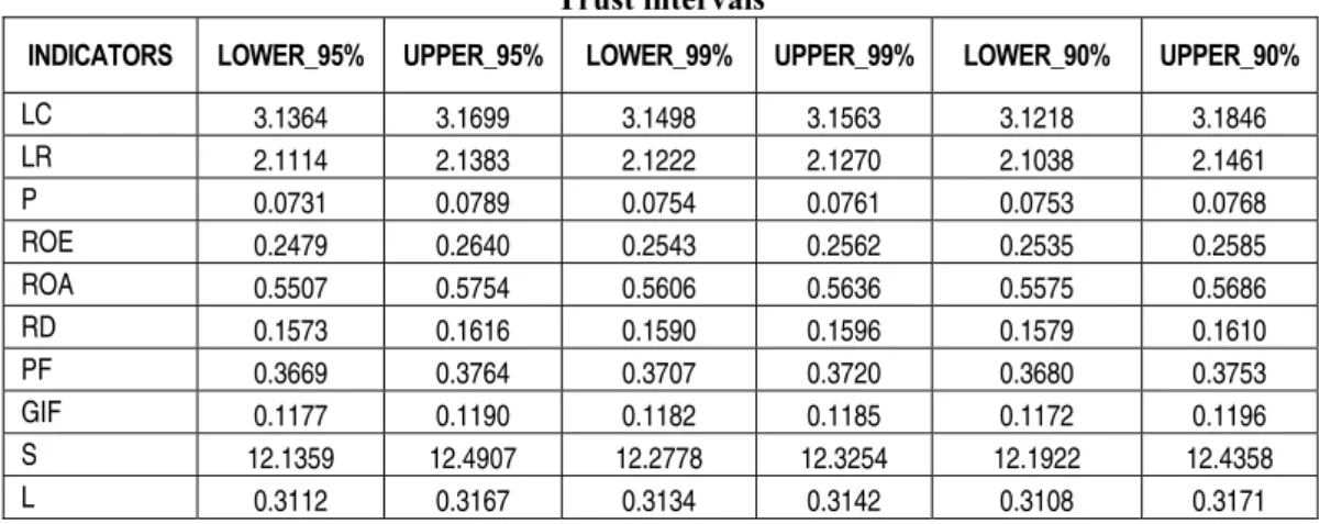
Test results show that KSN test-statistics value, for all analyzed indicators, is less than 1, and K (for a significant threshold, α, of 5%) is K0.95 equal to 1.3581. As KSN < K null test hypothesis can not be accepted, so there is no normal distribution of the analyzed indicators. But, following associated histograms a pronounced asymmetry has been observed and because n > 30 (n=40 enterprises) a N ( ;σ2/n) repartition can be accepted and we can proceed at determining trust intervals. In Table 1, trust intervals for these indicators are shown for different probabilities, δ:
Table 1 Trust intervals
INDICATORS LOWER_95% UPPER_95% LOWER_99% UPPER_99% LOWER_90% UPPER_90%
LC 3.1364 3.1699 3.1498 3.1563 3.1218 3.1846 LR 2.1114 2.1383 2.1222 2.1270 2.1038 2.1461 P 0.0731 0.0789 0.0754 0.0761 0.0753 0.0768 ROE 0.2479 0.2640 0.2543 0.2562 0.2535 0.2585 ROA 0.5507 0.5754 0.5606 0.5636 0.5575 0.5686 RD 0.1573 0.1616 0.1590 0.1596 0.1579 0.1610 PF 0.3669 0.3764 0.3707 0.3720 0.3680 0.3753 GIF 0.1177 0.1190 0.1182 0.1185 0.1172 0.1196 S 12.1359 12.4907 12.2778 12.3254 12.1922 12.4358 L 0.3112 0.3167 0.3134 0.3142 0.3108 0.3171
As expected, trust intervals are becoming larger as estimation accuracy, δ, increases (α = 1–δ). Because economic activity is subject to incertitude, investors have the possibility to use the following indicator’s average, as presented in Table 2, in order to fundament their investment decisions and correctly evaluate risks exposure.
Table 2 Average values
Indicators LC LR P ROE ROA RD PF GIF S L
Average value 3.1532 2.1249 0.0761 0.2560 0.5631 0.1595 0.3717 0.1184 12.3134 0.3140
Conclusions
Investigating risk at enterprise financial management level is a complex approach considering the multiple risk determination and risk sources diversity. Thus, risk areas have been identified (economic, financial, fiscal) and their afferent risk factors (cost structure, financial structure, fiscal regulations). After that, the research continued with risk evaluation, using statistical and mathematical methods, based upon elasticity coefficients and dispersion, both being a measurement for financial results indicators variability. Taking into consideration the business environment instability and its impact upon the financial indicators, the authors proceeded with trust interval determination for a set of financial indicators, interval that can be used in realizing financial predictions, accompanied by indicator’s average values, both for the sample and sector analyzed.
Acknowledgements
In this paper is disseminated as part of the research results obtained in the Exploratory Research Project PN-II-ID-PCE-2008-2, no.1764, CNCSIS, financed from the state budget through the Executor Unit for Superior Education and University Scientific Research Activity Financing, Romania.
References
Bauman, C., Schadewald, M. “Impact of foreign operations on reported effective tax rates: interplay of foreign taxes, US taxes and US GAAP”, Journal of International Accounting, Auditing & Taxation, 10, 2001, pp. 177-196
Becker, J., Fuest, C., Hemmelgarn, T., “Corporate Tax Reform and Foreign Direct Investment in Germany – Evidence from Firm-Level Data”, CESifo Working Paper Series 1722, CESifo Group Munich, 2006
Derashid, C., Zhang, H., “Effective tax rates and the “industrial policy” hypothesis: evidence from Malaysia”, Journal of International Accounting, Auditing & Taxation, 12, 2003, pp. 45-62
Dreze, J.H. (1987). Essays on Economic Decisions under Uncertainty, Cambridge University Press, Cambridge,
Gupta, S., Newberry, K., “Determinants of the Variability in Corporate Effective Tax Rates: Evidence from Longitudinal Data”, Journal of International Accounting and Public Policy, 16, 1997, pp. 1-34
Gil Lafuente, A.M. (1994). Analiza financiară în condiţii de incertitudine, AIT Laboratoires, Bucureşti
Kaufman A. (1994). Creativitatea în managementul întreprinderilor, AIT Laboratoires, Bucureşti
Mironiuc, M., “Metodologia de analiză a riscului economic pentru întreprinderea multiprodus”, Analele Ştiinţifice ale Universităţii „Alexandru Ioan Cuza” Iaşi, Tomul LII/LIII, 2005/2006
Nicodeme, G., “Computing effective corporate tax rates: comparisons and results”, MPRA Paper3808, 2001, University Library of Munich, Germany
Richardson, G., Lanis, R., “Determinants of the variability in corporate effective tax rates and tax reform: Evidence from Australia”, Journal of Accounting and Public Policy, 26, 2007, pp. 689-704
Md Noor, R., Fadzillah, N.S.M., Mastuki, N., “Corporate Tax Planning: A Study On Corporate Effective Tax Rates of Malaysian Listed Companies”, International Journal of Trade, Economics and Finance, Vol. 1, No. 2, August, 2010
Stancu, I. (2007). Finanţe, Editura Economică, Bucureşti
Vintilă, G. (2006). Gestiunea financiară a întreprinderii, Editura Didactică şi Pedagogică, Bucureşti