Bacteria in the global atmosphere – Part 2: Modelling of emissions and transport between different ecosystems

(1)

ACPD

9, 10829–10881, 2009

Bacterial emissions and transport

S. M. Burrows et al.

Title Page

Abstract Introduction

Conclusions References

Tables Figures

◭ ◮

Back Close

Full Screen / Esc

Printer-friendly Version

Interactive Discussion

Atmos. Chem. Phys. Discuss., 9, 10829–10881, 2009 www.atmos-chem-phys-discuss.net/9/10829/2009/ © Author(s) 2009. This work is distributed under the Creative Commons Attribution 3.0 License.

Atmospheric Chemistry and Physics Discussions

This discussion paper is/has been under review for the journalAtmospheric Chemistry and Physics (ACP). Please refer to the corresponding final paper inACPif available.

Bacteria in the global atmosphere –

Part 2: Modelling of emissions and

transport between di

_ff

erent ecosystems

S. M. Burrows, T. Butler, P. J ¨ockel, H. Tost, A. Kerkweg, U. P ¨oschl, and M. G. Lawrence

Max Planck Institute for Chemistry, Mainz, Germany

Received: 6 March 2009 – Accepted: 30 March 2009 – Published: 4 May 2009

Correspondence to: S. M. Burrows (susannah.burrows@mpic.de)

(2)

ACPD

9, 10829–10881, 2009

Title Page

Tables Figures

◭ ◮

Back Close

Full Screen / Esc

Abstract

Bacteria are constantly being transported through the atmosphere, which may have implications for human health, agriculture, cloud formation, and the dispersal of bac-terial species. We simulated the global transport of bacbac-terial cells, represented as 1µm diameter spherical solid particle tracers, in a chemistry-climate model. We

inves-5

tigated the factors influencing residence time and distribution of the particles, including emission region, CCN activity and removal by ice-phase precipitation. The global dis-tribution depends strongly on the assumptions made about uptake into cloud droplets and ice. The transport is also affected, to a lesser extent, by the emission region and by season. We examine the potential for exchange of bacteria between ecosystems

10

and obtain rough estimates of the flux from each ecosystem by using an optimal esti-mation technique, together with a new compilation of available observations described in a companion paper. Globally, we estimate the total emissions of bacteria to the at-mosphere to be 1400 Gg per year with an upper bound of 4600 Gg per year, originating mainly from grasslands, shrubs and crops. In order to improve understanding of this

15

topic, more measurements of the bacterial content of the air will be necessary. Future measurements in wetlands, sandy deserts, tundra, remote glacial and coastal regions and over oceans will be of particular interest.

1 Introduction

The transport of microorganisms in the atmosphere could have important implications

20

for several branches of science, including impacts on human health, agriculture, clouds, and microbial biogeography (Burrows et al., 2009). Unravelling these effects has been di_fficult, partly because so little is known about the concentrations and sources of at-mospheric microorganisms, as well as their transport pathways.

Bacteria are aerosolized from virtually all surfaces, including aerial plant parts, soil

25

(3)

ACPD

9, 10829–10881, 2009

Title Page

Tables Figures

◭ ◮

Back Close

Full Screen / Esc

from surfaces by gusts of wind or mechanical disturbances, such as shaking of leaves or surf breaking. Upon entering the air, they can be transported upwards by air currents and remain in the atmosphere for an average period of a few days. They are eventu-ally removed from the atmosphere by either “dry” deposition – adherence to buildings, plants, the ground and other surfaces in contact with the air – or “wet” deposition –

5

the precipitation of rain, snow or ice that has collected particles while forming or while falling to the surface.

The potential for bacteria and other microorganisms to be transported over long dis-tances through the air has long fascinated microbiologists and been a focus of the field of aerobiology. The average residence time of microorganisms in the atmosphere can

10

range from several days to weeks, long enough for cells to travel between continents. Many microorganisms have defense mechanisms which enable them to withstand the environmental stresses of air transport, including exposure to UV radiation, dessica-tion, and low pH within cloud water, so some microorganisms survive this long-range transport to new regions and arrive in a viable state.

15

We focus on the transport of bacteria through the air on global scales. Using a general circulation model to simulate particle transport (Sect. 2), we investigated the rate of transfer of bacteria-sized particles between various ecosystems. We estimated the emissions of bacteria from ten lumped ecosystem classes as a first step towards a simple model of emissions of biological particles to the atmosphere. An additional

20

advantage of this approach is that it allows us to investigate the transfer of genetic material between ecosystems, which has important implications for microbial biogeog-raphy. We give quantitative estimates of inter-ecosystem transport of bacteria, and show that it can be very large for some regions.

By adjusting the simulation results to observed concentrations, we estimated the

25

rate at which bacteria are transferred from land surfaces to the atmosphere. A realistic estimate of emission rates is an important step towards modelling realistic distributions in various regions.

(4)

ACPD

9, 10829–10881, 2009

Title Page

Tables Figures

◭ ◮

Back Close

Full Screen / Esc

troposphere could be similar to typical concentrations of atmospheric ice nuclei. Al-though most bacteria are not ice-nucleation active, this result suggests that the poten-tial for bacteria to play a significant role in ice nucleation deserves further investigation. Several investigators have used cloud microphysical models and cloud-resolving mod-els to study the potential e_ffects of bacteria on cloud development, but results of such

5

studies so far are inconclusive (Diehl et al., 2006; M ¨ohler et al., 2007).

2 Model description

We simulated particle transport using the EMAC model (ECHAM5/MESSy1.5 Atmo-spheric Chemistry). EMAC is a model system consisting of the atmoAtmo-spheric general circulation model ECHAM5 (Roeckner et al., 2003), coupled to various subprocess

10

models via the Modular Earth Submodel System (MESSy) interface (J ¨ockel et al., 2005; J ¨ockel et al., 2006). The system can be used to simulate both weather and climate, and study their effects on atmospheric chemistry and tracer transport. The model is available to the community (see http://www.messy-interface.org).

We simulated the transport of aerosol tracers of 1µm diameter and 1 g cm−3density.

15

A separate tracer was emitted from each of ten lumped ecosystem classes. Bacteria were emitted homogeneously within each region. This allowed us to determine the fate of particles from each ecosystem source region.

The model ran in T63L31 resolution for six simulated years without nudging of wind fields or other data assimilation. Initial meteorological fields were derived from the

20

ECMWF ERA-15 reanalysis for 1 January 1990. Monthly prescribed sea surface tem-perature were taken from the AMIP-II data set (Available from http://www-pcmdi.llnl. gov/). Initially, no bacteria were present in the air. The global atmospheric burden of the simulated bacteria reached quasi-equilibrium within the first three simulated years (spin-up). The analysis was conducted using climatological averages of the bacterial

25

distribution during the last three years of the simulation.

(5)

ACPD

9, 10829–10881, 2009

Title Page

Tables Figures

◭ ◮

Back Close

Full Screen / Esc

well as transport by advection and parameterized convection. A detailed description of the model set-up is included in Appendix A.

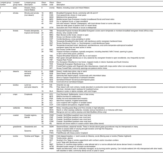
The ecosystem classification was based on the Olson World Ecosystems dataset (Olson, 1992) and is described in detail in Appendix B, Table B1. The choice of lumped ecosystem groups necessarily involves compromises. For the lumping used

5

here, taigas were grouped with tundras, since both are boreal, cold and usually frozen regions. However, some other snowy or boreal forests were grouped with forests, a group that also includes forests in tropical, sub-tropical and moderate climates. Other ambiguous ecosystem types include rice paddies (which could be considered crops or wetlands), mangroves and tidal mudflats (wetlands or coastal), and the various mixed

10

vegetation areas (such as field/woods types). Given the current limited state of knowl-edge regarding the emissions and distribution of bacteria in the air, it seemed appro-priate to limit the number of lumped classes to a reasonably small number.

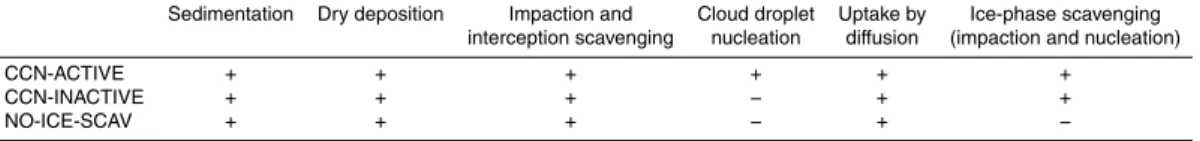
3 Sensitivity of modeled tracer transport to source ecosystem and scavenging

characteristics 15

Three model simulations were performed using different scavenging characteristics to investigate the e_ffects of scavenging processes on bacteria transport and lifetime. Losses to dry deposition, and to scavenging by impaction and interception were in-cluded in all three simulations, while CCN activity and ice phase scavenging were varied among the three sensitivity simulations: CCN-ACTIVE, CCN-INACTIVE and

20

NO-ICE-SCAV (Table 1).

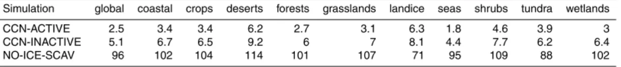
3.1 Global load and atmospheric lifetime

The mean global loads and lifetimes calculated for the three model simulations are given in Table 2. The lifetime of a few days for CCN-ACTIVE and CCN-INACTIVE bac-teria is consistent with theoretical expectations for particles of 1µm diameter (Roedel,

(6)

ACPD

9, 10829–10881, 2009

Title Page

Tables Figures

◭ ◮

Back Close

Full Screen / Esc

1992). In contrast, the long lifetimes of about 100 days for bacteria in the NO-ICE-SCAV simulation is unrealistically long.

3.1.1 Dependence of the global mean lifetime on source region and season

The global mean atmospheric lifetime of bacteria varies depending on the source re-gion (Table 2) and on season, due mainly to differences in transport and precipitation

5

patterns (Fig. 2).

Without ice phase scavenging, the mean lifetime is on the order of months, and the global NO-ICE-SCAV load varies relatively little during the year. In the CCN-INACTIVE simulation, particles originating in deserts, shrubs, grasslands, and coastal regions have the longest residence times, along with tundra and land ice particles during the

10

austral summer. Several of these ecosystems – deserts, shrubs, and grasslands – are predominantly located in drier, often tropical climates. Uptake into tropical convective systems and transport to the upper troposphere is likely, and low levels of precipita-tion in the source region result in slower removal, and long particle lifetimes. Particles emitted in these regions are therefore more likely to participate in long-distance

trans-15

port. Indeed, the long-distance transport of dust from warm deserts has long interested meteorologists. Bacteria are known to attach to dust particles and are routinely trans-ported over long distances within dust clouds, where the attenuation of UV radiation by the cloud is believed to improve chances of survival (Griffin et al., 2001a,b).

The source ecosystems with the shortest particle lifetimes in the CCN-INACTIVE

20

simulation are seas, tundra during the austral winter and spring, and forests.

(7)

ACPD

9, 10829–10881, 2009

Title Page

Tables Figures

◭ ◮

Back Close

Full Screen / Esc

3.2 Mean column density

The mean column density of the total bacteria is shown in Fig. 3. The CCN-INACTIVE and CCN-ACTIVE simulations, which both include ice phase scavenging, show very similar geographic distributions, with slightly higher concentrations in the CCN-INACTIVE simulation. In these two simulations, column densities are highest in

5

polar regions, consistent with the long lifetime of the land ice and tundra tracers (Fig. 2). High column densities in sub-Saharan Africa and northwestern Australia coincide with arid regions dominated by grasslands, shrubs and deserts, consistent with long particle lifetimes (deserts, shrubs) and large relative vertical transport rates (grasslands).

In the third simulation, NO-ICE-SCAV, column densities are much greater and more

10

homogeneous, consistent with the much longer lifetimes of particles in this simulation (Fig. 2). In the absence of efficient scavenging, the column densities are highest in the tropics, probably due to strong convective lifting, resulting in a longer lifetime. This interpretation is supported by studies of dust transport such as Schulz et al. (1998) which showed that satellite observations of dust plumes could only be reproduced with

15

a combination of the correct localization of source regions, rapid upward transport by convective updrafts and horizontal transport at upper altitudes.

4 Inversion

This section discusses the estimation of bacterial emissions in each ecosystem class based on a synthesis of literature results (Table 3) and model results. The analysis

20

is based on output from the CCN-ACTIVE simulation, which has the most realistic scavenging characteristics, including both CCN scavenging and ice-phase scavenging. Using literature estimates, we adjust the emissions of bacteria from each ecosys-tem to achieve a simulated distribution of airborne bacteria that is more representative of available observations. When sufficient information is available about the

distribu-25

(8)

ACPD

9, 10829–10881, 2009

Title Page

Tables Figures

◭ ◮

Back Close

Full Screen / Esc

techniques can be used to estimate sources (e.g. Kasibhatla et al., 2000). Given the paucity of data on bacterial concentrations, it seems reasonable to instead take a sim-pler approach to obtain some first estimates of the global sources and distribution. Our results give a starting point for further studies, and will be subject to modification and improvements as more measurements become available.

5

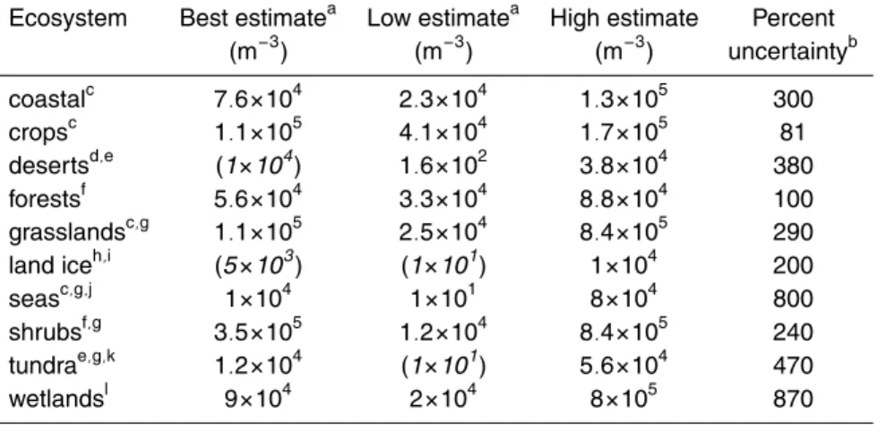
4.1 Observed concentrations

Our concentration estimates are presented in Table 3 and discussed in detail in a com-panion paper (Burrows et al., 2009). They are based mainly on the seven field studies listed in the footnotes of Table 3. Values are based on average concentrations of air-borne bacteria as observed over a period of a few days to a few weeks. In four of these

10

studies, only the culturable bacteria were observed. Culturable bacteria are typically measured by collecting aerosol samples on a nutrient agar and counting the number of colonies that form during subsequent incubation. In environmental aerosol samples, the culturable bacteria are typically about 1% of the total aerosol sample, although this fraction also depends on environmental and experimental variables (Burrows et al.,

15

2009). In three studies, total atmospheric bacteria were observed (Tong and Lighthart, 1999; Bauer et al., 2002; Harrison et al., 2005). Total bacteria can be counted by stain-ing proteins in an aerosol sample with a fluorescent dye, and then countstain-ing the number of bacteria in a sample under a microscope.

Observations are very sparse and even non-existant in some regions. To perform the

20

analysis, we made some additional assumptions about concentrations beyond those discussed in (Burrows et al., 2009). These are indicated by italic font and parentheses in Table 3, and explained in the footnotes to the table.

4.2 Mathematical considerations

In the present model, bacteria sources are constant and sinks depend linearly on

25

(9)

ACPD

9, 10829–10881, 2009

Title Page

Tables Figures

◭ ◮

Back Close

Full Screen / Esc

ecosystemmis given by a linear combination of the emission factorsf_nin theN ecosys-tems, weighted by a tensorW_{ni j kt} (the indicesi,j,k andt designating the model grid point in longitude, latitude, altitude, and time for each ecosystemm, respectively):

x_{mi j kt} ₌

N

X

n=1

W_{ni j kt}f_n. (1)

The tensorW_{ni j kt} is simply the distribution of bacteria from ecosystemn. Due to the

5

limited number of observations, the focus here will be only on values in the lowest model level, averaged in latitude, longitude and time, in which case Eq. (1) becomes

x_m₌

N

X

n=1

W_nmf_n, (2)

or, in vector notation,

x=Wf. (3)

10

The weighting functionWcan be calculated directly from the model results for emission at 1 m−2s−1. The weightsW_nm are then given by

W_nm ₌x_nm, (f=1) (4)

where x_nm is the mean concentration of the tracer from ecosystem n in ecosystem

m. Using these weights, which can be calculated from a single simulation, we can

15

calculate the distribution that would result from any arbitrary set of emission factors, (f_n). The inverse model can also be obtained directly fromW: if the emission factors

f_n are allowed to take on arbitrary real values, Eq. (3) has an exact solution (provided the matrixW is non-singular). It is also possible to find a best-fit solution under spe-cific constraints, such as requiring the fluxesf_n to be non-negative. Conceptually, this

20

(10)

ACPD

9, 10829–10881, 2009

Title Page

Tables Figures

◭ ◮

Back Close

Full Screen / Esc

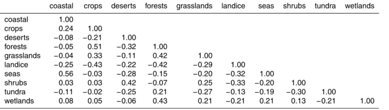
4.3 Discussion of the calculated weighting matrix and ecosystem

cross-correlations

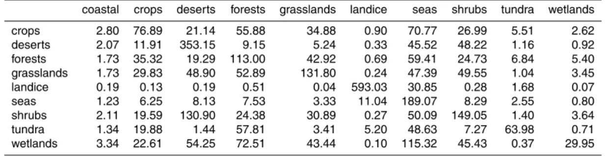
We calculated the weighting matrixWfor the simulated near-surface concentrations of the CCN-ACTIVE simulation (Table C1, Figs. 4, 5, and 6). Each row of Table C1 gives the mean concentrations of all ecosystems tracers found in the near-surface air of a

5

single destination ecosystem class, for homogeneous aerosol emissions of 1 m−2s−1. Some ecosystems have similar transport pathways and deposition footprints, result-ing in high correlations between the columns ofW. We computed the cross-correlations of the columns of W (Table C4 and Fig. 4). A large positive correlation between two ecosystems means that the distribution of the source ecosystem tracer among the ten

10

ecosystem classes is similar, as is likely to occur for geographically adjacent regions. Notable positive correlations occur between seas and coastal regions, which are al-ways contiguous, and between desert and shrub regions, which are almost alal-ways contiguous (Fig. 1). All other large positive correlations (correlation>0.4) involve the forest ecosystem tracer, whose distribution is positively correlated with the

distribu-15

tions of the crops, grasslands, and wetland tracers. Inspection of Fig. 1 shows that these ecosystems are indeed often found adjacent to forested regions.

A large cross-correlation between the distributions of two ecosystem tracers means that the tracer distributions are significantly linearly dependent on each other. This could point to weaknesses in the ecosystem lumping. For example, for future studies

20

it may be more meaningful to combine the coastal and seas regions, while splitting the forests into several groups that more accurately reflect the diversity of forested ecosystems. A sensible alternate subdivision, however, would ideally also take into account the availability of observations.

4.4 Numerical fitting procedures

25

(11)

ACPD

9, 10829–10881, 2009

Title Page

Tables Figures

◭ ◮

Back Close

Full Screen / Esc

exact solution, we fit the data iteratively while constraining fluxes to be non-negative. A first adjustment was done by hand to obtain a set of fluxes that meets this criterion, for the purposes of numerical optimization. Then a “best” fit (in a maximum likelihood sense) for the fluxes was obtained by using a constrained optimization technique.

4.4.1 Constrained weighted least squares fitting – Method 1

5

The solution was found by minimizing the weighted sum of the squared differences between modelled and literature fluxes:

N

X

n=1

(x_n−goal_n)2

high_n−low_n, (5)

where goaln is the fitting goal (literature estimate), subject to the constraint

f_n≥0 m−2s−1. The weighting term (high_n−low_n)−1reflects the uncertainty associated

10

with each literature estimate. Best-fit fluxes were calculated individually using the low, best and high literature estimates as the goal.

The minimization of the unweighted least-squares fit was also tested (results not shown). In the unweighted case, the highest estimated concentrations (grasslands, shrubs) were fitted with high precision, while the fits for other ecosystems (such as

15

forests and deserts) were relatively much poorer. The high-concentration regions dom-inated the fitting procedure such that the concentrations in other regions were seriously overestimated. Using the weighted cost function (Eq. 5) mitigates this problem, since regions with higher concentrations also tend to have greater associated absolute un-certainties.

20

4.4.2 Maximum likelihood fitting – Method 2

(12)

ACPD

9, 10829–10881, 2009

Title Page

Tables Figures

◭ ◮

Back Close

Full Screen / Esc

The following cost function was minimized:

N

X

n=1

(x_n−goal_n)2

(high_n−low_n) +µ·(exp(lown−xn)+exp(xn−highn)), (6) whereµis a scaling term for the boundary penalty, set to µ₌0.001, which is several orders of magnitude smaller than the first term in Eq. (6) for the values we used (given in Table 3). Maximum-likelihood parameters were calculated for the minimum, mean,

5

and maximum literature values, subject to the constraintf_n≥0 m−2s−1.

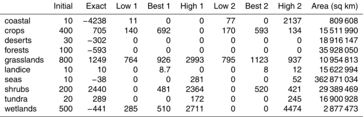
4.5 Results

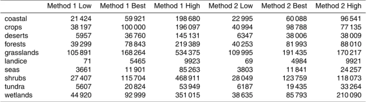
For the iterative optimization routines, an initial guess was selected by hand that satis-fied the upper and lower bounds on the mean concentration (the high and low literature estimates) and the lower bound on the fluxes (f_n≥0) for each ecosystem. The fitted

10

fluxes and the initial guess used in the numerical routines are listed in Table C3, while the modelled concentrations resulting from those fluxes are listed in Table C2. Addi-tionally, the estimated fluxes and resultant concentrations are illustrated in Fig. 7.

The exact solution of Eq. (3) for the literature best estimate of concentrations is listed in Table C31. For five of the ten ecosystem groups, the estimated mean fluxes

15

are negative, and at some locations, the resulting total bacterial concentrations are negative (not shown). Physically, concentrations can not be negative, and fluxes may be negative only if the model underestimates deposition (because modelled particle sinks are implicitly included in the weighting matrix W). If the concentrations being fitted had high precision, such a result could point to problems with the model, such

20

as a failure to accurately represent all model sinks. However, in the present case the

1

(13)

ACPD

9, 10829–10881, 2009

Title Page

Tables Figures

◭ ◮

Back Close

Full Screen / Esc

model transport and sink processes probably have a higher level of confidence than the highly uncertain literature estimates of bacterial aerosol concentrations.

In constrained fits (f >0), an exact fit to the best guess concentration cannot be at-tained, but the initial guess and the results of both fitting routines each produce concen-trations within the bounds of literature estimates for each of the ten ecosystem classes

5

(Fig. 7). The two fitting routines obtain similar results, with the exception of emissions from wetlands, which are 510 m−2s−1 in the Method 1 fit, and 0 in the Method 2 fit. The e_ffect of this di_fference on the resulting concentrations is small, as could be antici-pated considering the small impact of wetland emissions on concentrations elsewhere (Table C1).

10

The constrained iterative calculation of the best fit results in emissions greater than zero in only a few regions. The Method 2 best fit requires emissions from only four of ten ecosystem groups: grasslands, crops, shrubs and land ice. The Method 1 best fit additionally includes emissions from wetlands. With the exception of land ice, these are the ecosystems with the highest estimated bacterial concentrations. Fitted

con-15

centrations are lower than literature estimates in three regions (grasslands, crops, and shrubs), higher in five regions (coastal, deserts, forests, seas, and tundra) and close matches in two regions (land ice and wetlands). This observation makes clear why in certain regions, the estimated flux is zero in constrained fits and negative in uncon-strained fits. The emissions of grasslands, crops, and shrubs are fitted to values which

20

are not high enough to allow concentrations to be matched in the respective ecosys-tems. However, these tracers are exported to other ecosystems, such as deserts, in sufficient quantities that the literature estimates there are exceeded (Table C1). Addi-tional emissions from a region in which estimates are already exceeded would result in an even greater overshoot, further increasing the distance between the simulated

25

concentrations and the goal. The high emissions in grassland, crop, and shrub regions are a result of the numerical compromise between the competing goals of fitting high concentrations in those ecosystems and low concentrations elsewhere.

(14)

ACPD

9, 10829–10881, 2009

Title Page

Tables Figures

◭ ◮

Back Close

Full Screen / Esc

from the other ecosystem classes. The land ice ecosystem class is dominated by the Antarctic continent. The isolation of the continent from other land types is exacerbated in winter by the formation of the polar vortex. The result is a relatively small exchange of tracers with the seas, and virtually zero tracer exchange with other land ecosystems (Table C1). In addition, particles emitted here have a long lifetime (Fig. 2), so despite

5

low emission estimates, more than 90% of the aerosol found in the land ice regions is estimated to originate in that region.

In all other regions, contributions from the crop, grassland, and shrub tracers domi-nate, with these three sources making up about 80–90% or more of the near-surface load. An interesting feature is the high percentage of aerosol over the tundra that

orig-10

inates in agricultural areas. While tundra regions tend to be adjacent to forests and seas, these do not emit particles in the fitted model. Grasslands and shrubs, the other major emitters, are concentrated in warmer climates, and are thus often farther from tundra than agricultural areas.

Uncertainties were explored empirically by performing the inversion for an

ensem-15

ble of vectors with elements taken from the low, middle and high concentration esti-mates for each region (Fig. 8; see caption for details of the eensemble simluations). When fluxa values are unconstrained, Method 2 reproduces the exact solution, while Method 1 produces a different distribution with larger variability. This likely indicates that the Method 1 solution algorithm is more likely to be caught in a local minimum,

20

while the Method 2 constraint places a stronger penalty on solutions for which the con-centrations exceed the bounds of the estimated region, and is thus less likely to stray from the exact solution. Thus, Fig. 8 shows only the Method 2 solutions for constrained and unconstrained minimization.

Forcing the flux to be positive is equivalent to an a priori assumption that particle

25

deposition is simulated accurately. However, when negative fluxes are allowed, flux estimates in both forests and coastal regions are negative. A possible explanation is that model parameterizations underestimate particle deposition in these regions.

(15)

ACPD

9, 10829–10881, 2009

Title Page

Tables Figures

◭ ◮

Back Close

Full Screen / Esc

be robust. The largest uncertainties are found in wetlands and coastal regions, ecosys-tems with small land areas, which contribute little to the particle content of the air else-where. Thus, the emissions in these regions are poorly constrained by concentration estimates elsewhere.

Taking the median of the ensemble as the best estimate and the 5%ile–95%ile range

5

as an uncertainty estimate, we obtain about 1400 (22–4050) Gg year−1for the exact so-lution and about 690 (402–1488) Gg year−1for the Method 2 solution with the constraint that fluxes must be ≥0 (an overview of the percentile results is given in Appendix C, Tables C5 and C6). Because the positive constraint implies greater a priori knowledge than is available, we use the results of the exact solution ensemble as a best estimate

10

of the global emissions.

5 Analysis of adjusted model results

After adjusting the emissions to the Method 2 best fit values, the modelled particle distribution was recalculated. The total emissions from each of the ecosystems in the adjusted results are shown in Table 4. These emissions result in new patterns of

par-15

ticle distribution, with some differences to the distributions found in the homogeneous emissions case.

5.1 Distribution

5.1.1 Horizontal distribution

The change from homogeneous to adjusted emission fluxes results in a strong shift in

20

(16)

ACPD

9, 10829–10881, 2009

Title Page

Tables Figures

◭ ◮

Back Close

Full Screen / Esc

longest particle lifetimes. This means that they have a much larger impact on the vertical column density relative to their surface concentrations than the land ice or tundra tracers, which remain trapped near the surface.

5.2 Estimated global load and annual emissions

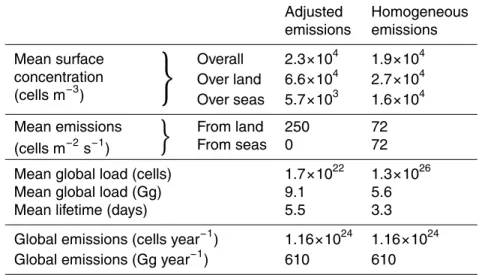
Overall diagnostics comparing the homogeneous emissions case and the adjusted

5

emissions case (using the Method 2 best fit) were calculated (Table 5). The elimina-tion of emissions from seas and oceans results in an increased difference between higher concentrations over land and lower concentrations over the seas. The global mean tracer lifetime is longer for the adjusted emissions case (5.5 days) than for the homogeneous emissions case (3.3 days).

10

For adjusted emissions, the estimated mean global load of bacterial cells is 1.7×1022. Assuming spherical bacteria of 1µm diameter and a density of 1 g cm−3, the mass of one cell is 0.52 pg and the total bacterial mass is approximately 9.0 Gg. The total estimated emission of bacterial cells from land surfaces is about 250 m−2s−1, resulting in total annual emissions of about 1.2×1024, or about 610 Gg. This is only

15

a very small fraction of the estimated total PBAP source of 1000 Tg/year (Jaenicke, 2005).

By comparison, Elbert et al. (2007) estimate that globally, fungal spores are emitted from land surfaces at an average rate of 200 m−2s−1over land, comparable to these results. However, with a mean assumed diameter of 5µm, a fungal spore has a mass of

20

about 65 pg, 125 times greater than the approximately 0.52 pg we assume for bacteria. Together, this results in a global fungal spore burden of about 140 Gg and a source of about 50 Tg per year. For the larger fungal spores, Elbert et al. (2007) assume a mean residence time of 1 day, while the bacteria we simulated have a mean residence time of 5.5 days.

(17)

ACPD

9, 10829–10881, 2009

Title Page

Tables Figures

◭ ◮

Back Close

Full Screen / Esc

5.3 Limitations and sources of uncertainty

The approach taken here amounts to the reduction of the global emission and transport of particles to a ten-box system, with sink processes and exchange between the boxes implicitly contained in the weighting matrix (Table C1). This approach allows useful insights to be gained into a problem for which the level of knowledge is, at present,

5

very low. However, such an approach has limitations, including the following:

– The ecosystem classification chosen involves various compromises (as discussed in Sect. 2) and some ecosystem classes may not be well-defined for the current purposes. For example, considering the high positive correlation of the coastal and seas tracer distributions (Table C4 and Fig. 4), it might be reasonable to

10

combine these groups. The forest group, on the other hand, includes a variety of diverse regions, and in a future study it might be more meaningful to distinguish between the various types of forest ecosystems.

– Most of the literature estimates are based on a single study or on assumptions about the similarities among ecosystem types. Even in well-studied land types

15

(such as croplands), the variability between sites is high, and the sites studied may not be representative of the entire class.

– Emissions of bacteria are likely to depend on temperature, wind, and other mete-orological variables (Jones and Harrison, 2004; Burrows et al., 2009), effects not considered in the current study. This may have important consequences for

dis-20

tributions (due, for instance, to differences between daytime and nighttime trans-port).

– The iterative fitting methods described in Sect. 4.4 may not produce unique solu-tions for the current problem.

– We consider spherical particles with a uniform diameter of 1µm, a typical size

25

(18)

ACPD

9, 10829–10881, 2009

Title Page

Tables Figures

◭ ◮

Back Close

Full Screen / Esc

long (Prescott et al., 1996). However, bacterial diameters can range from about 100 nm to as much as 750µm, and cells come in a variety of shapes (Schulz and Jorgensen, 2001). The size and shape of a bacterium will strongly affect its atmospheric lifetime.

In spite of these limitations, our approach takes advantage of the limited available

5

experimental data to yield first guesses of many values that so far have remained unquantified. This work provides a framework for the interpretation and incorporation of future experimental findings.

6 Summary and conclusions

6.1 Model results: particle transport characteristics

10

Using a global chemistry-climate model, we investigated the transport of bacteria in the atmosphere and its sensitivity to scavenging and the source ecosystem. While the ecosystem approach was applied here specifically to study emissions of bacteria, it also results in significant general learning about the differences in transport experi-enced by particles emitted from various ecosystems, and thus may be applicable to

15

other natural organic aerosols.

We estimate the mean global atmospheric lifetime of a homogeneously emitted bac-teria tracer to be about 2.5 days for the ACTIVE simulation, 5 days for CCN-INACTIVE, and several months for NO-ICE-SCAV. These lifetimes are long enough for significant long-distance transport to occur in the atmosphere. For tracers with the

20

(19)

ACPD

9, 10829–10881, 2009

Title Page

Tables Figures

◭ ◮

Back Close

Full Screen / Esc

6.2 Estimation of global emissions of bacterial aerosol

The results of a literature review (Burrows et al., 2009) and the modeling study were synthesized to obtain a better understanding of the global distribution of bacteria in the atmosphere. Using a maximum likelihood estimation procedure, we estimated emission rates for each of ten ecosystem types. The mean continental emissions of

5

bacteria were estimated to be about 250 cells m−2s−1 or 610 Gg year−1 by an itera-tive method with fluxes constrained to be posiitera-tive. By estimating the emissions for an ensemble of estimated concentrations, we obtain total global emissions of 1400 (20– 4000) Gg year−1(median and 5%ile–95%ile), consistent with literature measurements showing concentrations to be about 104–105m−3 in most regions. This is, based on

10

the broad range of literature reviewed, the first estimate of global bacterial emissions to the atmosphere.

The estimated emissions are of the same order of magnitude by number as fungal spore emissions, which Elbert et al. (2007) estimated to be about 200 m−2s−1. The mass flux, however, is much smaller than the 50 Tg/year estimated for total fungal

15

spores, because the mass of a bacterium, assumed here to be 0.52 pg/cell, is much smaller than that of a single spore, assumed by Elbert et al. (2007), to be 65 pg. The estimate of fungal spore emissions by Elbert et al. (2007), in turn, is small compared to the the 1000 Tg/year (Jaenicke, 2005) that have been estimated for the total emission of primary biological aerosol particles.

20

Sources of bacteria in the adjusted simulation were mainly restricted to the regions with the highest estimated bacterial concentrations (grasslands, shrubs and crops). Strong emissions in those regions meant that particles were exported in quantities large enough to exceed estimated mean concentrations elsewhere.

6.3 Outlook

25

(20)

ACPD

9, 10829–10881, 2009

Title Page

Tables Figures

◭ ◮

Back Close

Full Screen / Esc

– How important is “continuous” vs. “intermittent” transport of bacteria (e.g. Wolfen-barger, 1946)?

– How do bacteria influence cloud formation? Does the presence of bacteria affect precipitation or the radiative properties of clouds as part of a larger feedback cycle (the “bioprecipitation” hypothesis) (Schnell and Vali, 1973; Sands et al., 1992;

5

Bauer et al., 2003; Morris et al., 2005; Sun and Ariya, 2006)?

– To what degree are bacteria able to reproduce in the atmosphere? Does the atmosphere provide a niche for particular microorganisms (Dimmick et al., 1979; Sattler et al., 2001; Amato et al., 2007)?

– Does the degradation of organic compounds by bacteria play a significant role

10

in the chemistry of liquid particles in the atmosphere (Herlihy et al., 1987; Ariya, 2002; Amato et al., 2007)?

The answer to each of these questions either depends on or enhances our knowledge of atmospheric bacterial concentrations. Quantifying the distribution of atmospheric bacteria will therefore remain an important goal of investigators seeking to understand

15

interactions between bacteria and the atmospheric environment. Attention should be paid to quantifying total (as opposed to culturable) bacterial concentrations, emission fluxes and vertical profiles. Flux measurements of total bacteria are especially impor-tant for improving understanding of the origins of airborne bacteria.

Past measurements of ambient bacterial concentration have tended to focus on

ur-20

ban sites and point sources, or on emissions from agricultural sources. As a result, many ecosystems have been neglected, especially those that are not easily acces-sible to researchers. Ecosystem types for which no published measurements of air-borne bacterial concentrations were found include tropical rain-forests, wetlands, sandy deserts, tundra, and glaciated regions. Also, few measurements have been made over

25

(21)

ACPD

9, 10829–10881, 2009

Title Page

Tables Figures

◭ ◮

Back Close

Full Screen / Esc

whether the marine source makes a significant contribution to the high IN concentra-tions observed in these regions as argued by Schnell and Vali (1976).

Further laboratory measurements are needed to investigate the activity of bacteria in droplet and ice crystal formation. While it is clear that some bacteria are highly effective ice nucleators, it remains unclear what percentage of environmental bacteria are

IN-5

active or how to treat the CCN activity of environmental bacteria (CCN activities have been measured by Bauer et al., 2003 and Franc and DeMott, 1998). Studies address-ing uptake into cloud and rain droplets would help to quantify scavengaddress-ing e_fficiency for bacterial cells, and the potential effect of hydrophobic cell surfaces on uptake.

The microbiology of the atmosphere is a topic that presents challenges and

oppor-10

tunities for many disciplines. Atmospheric transport models can make a useful con-tribution to understanding the sources and discon-tribution of bacteria in the atmosphere. However, there is a need for more measurements, particularly measurements of total (as opposed to viable) bacterial concentrations and fluxes, if further progress it to be made. Because of the many gaps in current knowledge of atmospheric microflora, this

15

study can not be considered complete. Nevertheless, it is expected that the global overview obtained from the current approach, and the estimates of the mean global emissions and concentrations, should be useful in assessing the likely magnitude of effects resulting from the presence of bacteria in the air.

Appendix A Model setup and data handling

20

A1 Tracers in EMAC

In the EMAC system, the back-end for consistent handling of atmospheric con-stituents is the generic submodel TRACER (J ¨ockel et al., 2008), which includes two sub-submodels, TRACER FAMILY and TRACER PDEF. The sub-submodel TRACER FAMILY was used to correct small nonlinearities in tracer advection due to

25

(22)

ACPD

9, 10829–10881, 2009

Title Page

Tables Figures

◭ ◮

Back Close

Full Screen / Esc

due to numerical overshoots. The submodel PTRAC was used to define the tracers and their characteristics, including size, density, and CCN activity.

Tracer advection is calculated in EMAC using the Lin and Rood (1996) integration algorithm, which is mass-conserving, linear, and monotonic in its 1-D form.

The EMAC submodel ONLEM (Kerkweg et al., 2006b,c) enables flexible online

cal-5

culation of tracer emissions based on a combination of geographical data (e.g. land cover or soil type) and/or current meteorological conditions. ONLEM was extended by a subroutine to simulate the emission of the bacteria tracer.

Sedimentation and other dry deposition processes are simulated by the MESSy sub-models SEDI and DRYDEP, respectively (Kerkweg et al., 2006a), while wet deposition

10

is simulated by the MESSy submodel SCAV (Tost et al., 2006).

A2 Dry deposition and sedimentation

The EMAC parameterization of dry deposition in the submodel DRYDEP is docu-mented in Kerkweg et al. (2006a). Dry deposition is calculated online, considering the effects of Brownian diffusion, impaction and interception onto vegetation, water, bare

15

soil and snow surfaces. Dry deposition on vegetation is calculated using the “big-leaf” approach (Hicks et al., 1987), as parameterized by Slinn (1982) and later modified by Gallagher et al. (2002). Dry deposition on water surfaces is calculated following Slinn and Slinn (1980) over smooth waters and Hummelshøj et al. (1992) over choppy wa-ters. Dry deposition over bare soil and snow surfaces is calculated according to Slinn

20

(1976).

Dry deposition due to surface interactions only occurs in the lowest model layer, as opposed to sedimentation, which occurs throughout the model and is independent of surface characteristics. For these reasons, sedimentation is treated separately in EMAC, in the SEDI submodel (Kerkweg et al., 2006a). The settling velocity is given by

25

(23)

ACPD

9, 10829–10881, 2009

Title Page

Tables Figures

◭ ◮

Back Close

Full Screen / Esc

A3 Wet deposition

The wet deposition parameterizations used in EMAC are documented in Tost et al. (2006) and Tost (2006). Aerosol scavenging rates were calculated online, in depen-dence on cloud droplet and raindrop size, rainfall and snowfall intensity and aerosol diameter.

5

A3.1 Scavenging during cloud droplet nucleation and growth

The uptake of aerosol particles into cloud droplets due to nucleation on the particles is parameterized by an empirical function for the scavenged fraction, which was derived from measurements presented by Svenningsson et al. (1997) and Martinsson et al. (1999). The nucleation rate for CCN-active particles rises sharply from less than 1%

10

forr_aer₌0.1µmto 50% atr_aer₌0.2µmand over 99% atr_aer₌0.4µm. The particles in this study have a radius of 1µm, and so are entirely taken up into cloud droplets if assumed to be CCN-active. CCN-inactive particles are not taken up by nucleation scavenging.

A3.2 Scavenging by falling raindrops

To estimate scavenging by falling raindrops (both within and below the cloud), SCAV

15

uses a semi-empirical parameterization of the collision efficiency E first proposed by Slinn (1983), that includes the effects of Brownian diffusion, interception and impaction scavenging. Its applicability has also been demonstrated by Andronache (2003, 2004). Removal by impaction and interception scavenging during transport to the upper tro-posphere is inefficient for the 1µm particles considered in this study. This is because

20

(24)

ACPD

9, 10829–10881, 2009

Title Page

Tables Figures

◭ ◮

Back Close

Full Screen / Esc

A3.3 Impaction scavenging by frozen hydrometeors

Although scavenging by falling raindrops is inefficient, impaction scavenging by falling snow and ice is significant, which contributes to the large differences in the simula-tions with and without ice-phase scavenging. The scavenging coe_fficient for impaction scavenging by snow and ice is set to 0.1.

5

A3.4 Nucleation scavenging by frozen hydrometeors

The ice content of clouds is represented in EMAC by a single bulk variable. For nu-cleation scavenging by ice, a constant scavenging ratio is applied (the same approach used in e.g. Stier et al., 2005). For mixed-phase clouds warmer than 238.15 K (−35◦C), the scavenging coefficient is set to 0.8; otherwise it is set to 0.05. A smaller fraction of

10

the aerosol is scavenged in mixed-phase clouds than in warm clouds. This has been attributed to the Bergeron-Findeisen effect, which leads to growth of a small number of ice crystals at the expense of the evaporation of a larger number of cloud droplets, which release particles (Henning et al., 2004).

Ice phase scavenging was found to be an important removal process, but it is poorly

15

understood at present and its representation in models is crude. For instance, dif-ferential scavenging due to the different ice-nucleating capabilities of particles is not considered in the model. Since bacteria are often good ice nucleators, they may be scavenged at higher rates than other aerosol particles, but this effect could not be con-sidered in the current study. Future work is necessary to understand the sensitivity of

20

simulated aerosol distributions to ice-phase scavenging rates and to develop improved scavenging parameterizations.

A3.5 Large scale clouds, deep convection, and vertical diffusion

In the model set-up used for this study, the vertical transport was parameterized with the submmodel CVTRANS. Cumulus convection is calculated via the mass flux

(25)

ACPD

9, 10829–10881, 2009

Title Page

Tables Figures

◭ ◮

Back Close

Full Screen / Esc

scheme of Tiedtke (1989) with modifications for penetrative convection according to Nordeng (1994). Stratiform cloud microphysics is calculated using the parameteriza-tion of Lohmann and Roeckner (1996) and the statistical cloud cover scheme of Tomp-kins (2002). The turbulent vertical flux in the boundary layer is calculated according to Roeckner et al. (2003), Chapter 5.

5

A4 Data handling

Model results were output as averages over each six-hour time interval. In post-processing, this output was averaged to obtain “climatological” monthly mean values for mixing ratios and loss rates in each grid cell2. The analysis was done on the ba-sis of the monthly mean data. Finally, ecosystem emission fluxes were adjusted to

10

fit estimated concentrations from the literature. The numerical procedures used are described in Sect. 4.

The inversion analysis was performed using the open-source statistical program-ming language R and its standard libraries (R Development Core Team, 2008). For the Method 1 fitting, the method of Byrd et al. (1995) was used (as implemented in

15

the R statistics function optim), which finds local minima of a single-valued function while satisfying upper and lower boundary conditions on each function argument. In Method 2, the cost function was minimized using a constrained nonlinear optimization function from the R statistics package (nlminb), which utilizes the routines from the PORT library developed at AT&T Bell Laboratories (Gay, 1990).

20

2

(26)

ACPD

9, 10829–10881, 2009

Title Page

Tables Figures

◭ ◮

Back Close

Full Screen / Esc

Appendix B Ecosystem lumping

The basis for ecosystem classification is the Olson World Ecosystems dataset (Olson, 1992), which is freely available from NOAA at the time of writing (http://www.ngdc.noaa. gov/ecosys/). Ecosystem classes are assigned at each point of a grid with a mixture of 30 min and 10 min spatial resolution. Each class is associated with an integer index

5

from 0 through 73 (inclusive), with 14 of the indices remaining unused.

Because the Olson ecosystem classification was too detailed for the present pur-poses, the classes were lumped into groups as detailed in Table B1. The geographic distribution of the lumped ecosystems is illustrated in Fig. 1. The data were regridded onto the model grid points using NCREGRID (J ¨ockel, 2006). For each box of the new

10

grid, NCREGRID returns a vector. Each element of the vector is the fraction of the new grid box covered by one ecosystem from the lumped set (see regridding type IFX in J ¨ockel, 2006).

Appendix C Tabulated results

See Tables C1–C6.

15

Acknowledgements. This material is based upon work supported under a National Science Foundation Graduate Research Fellowship (grant number 0633824) awarded to Susannah Burrows. The Max Planck Institute for Chemistry and the International Max Planck Research School on atmospheric chemistry and physics are acknowledged gratefully for hosting Susannah Burrows’ research.

20

(27)

ACPD

9, 10829–10881, 2009

Title Page

Tables Figures

◭ ◮

Back Close

Full Screen / Esc

References

Amato, P., Demeer, F., Melaouhi, A., Fontanella, S., Martin-Biesse, A.-S., Sancelme, M., Laj, P., and Delort, A.-M.: A fate for organic acids, formaldehyde and methanol in cloud water: their biotransformation by micro-organisms, Atmos. Chem. Phys., 7, 4159–4169, 2007, http://www.atmos-chem-phys.net/7/4159/2007/. 10848

5

Andronache, C.: Estimated variability of below-cloud aerosol removal by rainfall for observed aerosol size distributions, Atmos. Chem. Phys., 3, 131–143, 2003,

http://www.atmos-chem-phys.net/3/131/2003/. 10851

Andronache, C.: Estimates of sulfate aerosol wet scavenging coefficient for locations in the Eastern United States, Atmos. Environ., 38, 795–804, 2004. 10851

10

Ariya, P.: Microbiological degradation of atmospheric organic compounds, Geophys. Res. Lett., 29, p. 34, doi:10.1029/2002GL015637, 2002. 10848

Bauer, H., Kasper-Giebl, A., L ¨oflund, M., Giebl, H., Hitzenberger, R., Zibuschka, F., and Puxbaum, H.: The contribution of bacteria and fungal spores to the organic carbon con-tent of cloud water, precipitation and aerosols, Atmos. Res., 64, 109–119, doi:10.1016/ 15

S0169-8095(02)00084-4, 2002. 10836, 10863

Bauer, H., Giebl, H., Hitzenberger, R., Kasper-Giebl, A., Reischl, G., Zibuschka, F., and Puxbaum, H.: Airborne bacteria as cloud condensation nuclei, J. Geophys. Res., 108, 4658, doi:10.1029/2003JD003545, 2003. 10848, 10849

Burrows, S. M., Elbert, W., Lawrence, M., and P ¨oschl, U.: Bacteria in the global atmosphere – 20

Part 1: Review and synthesis of literature data for different ecosystems, Atmos. Chem. Phys. Discuss., 9, 10777–10827, 2009,

http://www.atmos-chem-phys-discuss.net/9/10777/2009/. 10830, 10836, 10845, 10847, 10863

Byrd, R., Lu, P., Nocedal, J., and Zhu, C.: A limited memory algorithm for bound constrained 25

optimization, SIAM J. Sci. Stat. Comp., 16, 1190–1208, 1995. 10853

Diehl, K., Simmel, M., and Wurzler, S.: Numerical sensitivity studies on the impact of aerosol properties and drop freezing modes on the glaciation, microphysics, and dynamics of clouds, J. Geophys. Res., 111, 7202, doi:10.1029/2005JD005884, 2006. 10832

Dimmick, R., Wolochow, H., and Chatigny, M.: Evidence for more than one division of bacteria 30

within airborne particles, Appl. Environ. Microb., 38, 642–643, 1979. 10848

(28)

ACPD

9, 10829–10881, 2009

Title Page

Tables Figures

◭ ◮

Back Close

Full Screen / Esc

biogenic aerosols in the atmosphere: wet and dry discharged spores, carbohydrates, and inorganic ions, Atmos. Chem. Phys., 7, 4569–4588, 2007,

http://www.atmos-chem-phys.net/7/4569/2007/. 10844, 10847

Enting, I.: Inverse Methods in Global Biogeochemical Cycles, chap. Green’s function methods of tracer inversion, American Geophysical Union, 2000. 10837

5

Franc, G. and DeMott, P.: Cloud Activation Characteristics of Airborne Erwinia carotovora Cells, J. Appl. Meteorol., 37, 1293–1300, 1998. 10849

Gallagher, M., Nemitz, E., Dorsey, J., Fowler, D., Sutton, M., Flynn, M., and Duyzer, J.: Mea-surements and parameterizations of small aerosol deposition velocities to grassland, arable crops, and forest: Influence of surface roughness length on deposition, J. Geophys. Res., 10

107(D12), 4154, doi:10.1029/2001JD000817, 2002. 10850

Gay, D.: Usage summary for selected optimization routines, Computing Science Technical Report, AT&T Bell Laboratories, 1990. 10853

Gregory, P.: The microbiology of the atmosphere, Leonard Hill, USA, 1973. 10830

Griffin, D., Garrison, V., Herman, J., and Shinn, E.: African desert dust in the Caribbean atmo-15

sphere: Microbiology and public health, Aerobiologia, 17, 203–213, 2001a. 10834

Griffin, D., Kellogg, C., and Shinn, E.: Dust in the Wind: Long Range Transport of Dust in the Atmosphere and Its Implications for Global Public and Ecosystem Health, Global Change & Human Health, 2, 20–33, 2001b. 10834

Griffin, D., Westphal, D., and Gray, M.: Airborne microorganisms in the African desert dust 20

corridor over the mid-Atlantic ridge, Ocean Drilling Program, Leg 209, Aerobiologia, 22, 211– 226, 2006. 10863

Harrison, R., Jones, A., Biggins, P., Pomeroy, N., Cox, C., Kidd, S., Hobman, J., Brown, N., and Beswick, A.: Climate factors influencing bacterial count in background air samples, Int. J. Biometeorol., 49, 167–178, 2005. 10836, 10863

25

Henning, S., Bojinski, S., Diehl, K., Ghan, S., Nyeki, S., Weingartner, E., Wurzler, S., and Baltensperger, U.: Aerosol partitioning in natural mixed-phase clouds, Geophys. Res. Lett., 31, L06101, doi:10.1029/2003GL019025, 2004. 10852

Herlihy, L., Galloway, J., and Mills, A.: Bacterial utilization of formic and acetic acid in rainwater, Atmos. Environ., 21, 2397–2402, 1987. 10848

30

(29)

ACPD

9, 10829–10881, 2009

Title Page

Tables Figures

◭ ◮

Back Close

Full Screen / Esc

Hinds, W. C.: Aerosol technology: Properties, behavior, and measurement of airborne parti-cles, Wiley-Interscience, New York, USA, 442 pp., 1982. 10850

Hummelshøj, P., Jensen, N., and Larson, S.: Precipitation scavenging and atmosphere-surface exchange, chap. Particle dry deposition to a sea surface, Hemisphere Publishing Corpora-tion, Washington, USA, 1992. 10850

5

Jaenicke, R.: Abundance of Cellular Material and Proteins in the Atmosphere, Science, 308, p. 73, doi:10.1126/science.1106335, 2005. 10844, 10847

J ¨ockel, P.: Technical note: Recursive rediscretisation of geo-scientific data in the Modular Earth Submodel System (MESSy), Atmos. Chem. Phys., 6, 3557–3562, 2006,

http://www.atmos-chem-phys.net/6/3557/2006/. 10854 10

J ¨ockel, P., Sander, R., Kerkweg, A., Tost, H., and Lelieveld, J.: Technical Note: The Modular Earth Submodel System (MESSy) - a new approach towards Earth System Modeling, Atmos. Chem. Phys., 5, 433–444, 2005,

J ¨ockel, P., Tost, H., Pozzer, A., Br ¨uhl, C., Buchholz, J., Ganzeveld, L., Hoor, P., Kerk-15

weg, A., Lawrence, M. G., Sander, R., Steil, B., Stiller, G., Tanarhte, M., Taraborrelli, D., van Aardenne, J., and Lelieveld, J.: The atmospheric chemistry general circulation model ECHAM5/MESSy1: consistent simulation of ozone from the surface to the mesosphere, At-mos. Chem. Phys., 6, 5067–5104, 2006,

http://www.atmos-chem-phys.net/6/5067/2006/. 10832 20

J ¨ockel, P., Kerkweg, A., Buchholz-Dietsch, J., Tost, H., Sander, R., and Pozzer, A.: Technical Note: Coupling of chemical processes with the Modular Earth Submodel System (MESSy) submodel TRACER, Atmos. Chem. Phys., 8, 1677–1687, 2008,

Jones, A. M. and Harrison, R. M.: The effects of meteorological factors on atmospheric 25

bioaerosol concentrations – a review, Sci. Total Environ., 326, 151–180, 2004. 10830, 10845 Kasibhatla, P., Heimann, M., Rayner, P., Mahowald, N., Prinn, R., and Hartley, D.(eds.): Inverse

Methods in Global Biogeochemical Cycles, American Geophysical Union, 2000. 10836 Kerkweg, A., Buchholz, J., Ganzeveld, L., Pozzer, A., Tost, H., and J ¨ockel, P.: Technical Note:

An implementation of the dry removal processes DRY DEPosition and SEDImentation in 30

the Modular Earth Submodel System (MESSy), Atmos. Chem. Phys., 6, 4617–4632, 2006a. 10850

(30)

Chem-ACPD

9, 10829–10881, 2009

Title Page

Tables Figures

◭ ◮

Back Close

Full Screen / Esc

istry Department, Max-Planck Institute of Chemistry, PO Box 3060, 55020 Mainz, Germany, online available: akerkweg@mpch-mainz.mpg.de, 2006b. 10850

Kerkweg, A., Sander, R., Tost, H., and J ¨ockel, P.: Technical note: Implementation of prescribed (OFFLEM), calculated (ONLEM), and pseudo-emissions (TNUDGE) of chemical species in the Modular Earth Submodel System (MESSy), Atmos. Chem. Phys., 6, 3603–3609, 2006c. 5

10850

Lighthart, B. and Shaffer, B. T.: Bacterial flux from chaparral into the atmosphere in mid-summer at a high desert location, Atmos. Environ., 28, 1267–1274, 1994. 10863

Lin, S. and Rood, R.: Multidimensional Flux-Form Semi-Lagrangian Transport Schemes, Monthly Weather Review, 124, 2046–2070, 1996. 10850

10

Lohmann, U. and Roeckner, E.: Design and performance of a new cloud microphysics scheme developed for the ECHAM general circulation model, Clim. Dynam., 12, 557–572, 1996. 10853

Martinsson, B., Frank, G., Cederfelt, S., Swietlicki, E., Berg, O., Zhou, J., Bower, K., Bradbury, C., Birmili, W., Stratmann, F., et al.: Droplet nucleation and growth in orographic clouds in 15

relation to the aerosol population, Atmos. Res., 50, 289–315, 1999. 10851

M ´ohler, O., DeMott, P. J., Vali, G., and Levin, Z.: Microbiology and atmospheric processes: the role of biological particles in cloud physics, Biogeosciences, 4, 1059–1071, 2007,

http://www.biogeosciences.net/4/1059/2007/. 10832

Morris, C., Georgakopoulos, D., and Sands, D.: Ice nucleation active bacteria and their potential 20

role in precipitation, J. Phys. IV France, 121, 87–103, 2005. 10848

Nordeng, T. E.: Extended versions of the convective parameterization scheme at ECMWF and their impact on the mean and transient activity of the model in the tropics., Tech. Rep. Technical Memorandum 206, ECMWF, Reading, UK, 1994. 10853

Olson, J.: World ecosystems (WE1. 4): Digital raster data on a 10 minute geographic 1080 25

(2160 grid square), Global Ecosystem Database, Version, 1, 1992. 10833, 10854, 10866, 10873

Prescott, L., Harley, J., and Klein, D.: Microbiology, Wm. C. Brown Publishers, Dubuque, IA, USA, third edn., 37–41, 1996. 10846

R Development Core Team: R: A Language and Environment for Statistical Computing, version 30

2.7.2, R Foundation for Statistical Computing, Vienna, Austria, online available at: http:// www.R-project.org, ISBN 3-900051-07-0, 2008. 10853

(31)

ACPD

9, 10829–10881, 2009

Title Page

Tables Figures

◭ ◮

Back Close

Full Screen / Esc

S., Kirchner, I., Kornblue, L., Manzini, E., et al.: The atmospheric general circulation model ECHAM5. Part 1: Model description, Tech. Rep. 349, Max Planck Institute for Meteorology, Hamburg, Germany, 2003. 10832, 10853

Roedel, W.: Physik unserer Umwelt, Die Atmosph ¨are, Berlin Heidelberg, Germany, 1992. 10833

5

Sands, D., Langhans, V., Scharen, A., and Desmet, G.: The association between bacteria and rain and possible resultant meteorological implications, Idojaras (Budapest), 86, 148–152, 1992. 10848

Sattler, B., Puxbaum, H., and Psenner, R.: Bacterial growth in supercooled cloud droplets, Geophys. Res. Lett., 28, 239–242, doi:10.1029/2000GL011684, 2001. 10848

10

Schnell, R. and Vali, G.: World-wide source of leaf-derived freezing nuclei, Nature, 246, 212– 213, 1973. 10848

Schnell, R. and Vali, G.: Biogenic Ice Nuclei: Part I. Terrestrial and Marine Sources, J. Atmos. Sci., 33, 1554–1564, 1976. 10849

Schulz, H. and Jorgensen, B.: Big Bacteria, Annu. Rev. Microbiol., 55, 105–137, 2001. 10846 15

Schulz, M., Balkanski, Y. J., Guelle, W., and Dulac, F.: Role of aerosol size distribu-tion and source locadistribu-tion in a three-dimensional simuladistribu-tion of a Saharan dust episode tested against satellite-derived optical thickness, J. Geophys. Res., 103, 10579–10592, doi: 10.1029/97JD02779, 1998. 10835

Shaffer, B. T. and Lighthart, B.: Survey of Culturable Airborne Bacteria at Four Diverse Lo-20

cations in Oregon: Urban, Rural, Forest, and Coastal, Microb. Ecol., 34, 167–177, 1997. 10863

Slinn, S. and Slinn, W.: Predictions for Particle Deposition on Natural Waters, Atmos. Environ., 14, 1013–1016, doi:10.1016/0004-6981(80)90032-3, 1980. 10850

Slinn, W.: Predictions for particle deposition to vegetative canopies, Atmos. Environ., 16(7), 25

1785–1794, doi:10.1016/0004-6981(82)90271-2, 1982. 10850

Slinn, W.: Precipitation Scavenging, Dry Deposition and Resuspension, chap. chap. 11, Pre-cipitation Scavenging, United States Dept. of Energy, 1983. 10851

Slinn, W. G. N.: Atmosphere-surface exchange of particulate and gaseous pollutants, chap. Dry deposition and resuspension of aerosol particles – a new look at some old problems, US 30

DOE Tech. Info. Center, Oak Ridge, TN, USA, 1976. 10850