Iterative Approximation of Basic Belief
Assignment Based on Distance of Evidence
Yi Yang*, Yuanli Liu
SKLSVMS, School of Aerospace, Xi’an Jiaotong University, Xi’an, Shaanxi, China 710049 *[email protected]
Abstract
In the theory of belief functions, the approximation of a basic belief assignment (BBA) is for reducing the high computational cost especially when large number of focal elements are available. In traditional BBA approximation approaches, a focal element’s own characteris-tics such as the mass assignment and the cardinality, are usually used separately or jointly as criteria for the removal of focal elements. Besides the computational cost, the distance between the original BBA and the approximated one is also concerned, which represents the loss of information in BBA approximation. In this paper, an iterative approximation approach is proposed based on maximizing the closeness, i.e., minimizing the distance between the approximated BBA in current iteration and the BBA obtained in the previous iteration, where one focal element is removed in each iteration. The iteration stops when the desired number of focal elements is reached. The performance evaluation approaches for BBA approximations are also discussed and used to compare and evaluate traditional BBA approximations and the newly proposed one in this paper, which include traditional time-based way, closeness-time-based way and new proposed ones. Experimental results and related analyses are provided to show the rationality and efficiency of our proposed new BBA approximation.
Introduction
The theory of belief functions [1], also called Dempster-Shafer theory (DST), has many advan-tages in uncertainty modeling and reasoning [2,3]; however, it has also been argued due to its limitations [4,5]. One of the limitation is the high computational cost encountered in the pro-cedure such as the evidence combination, conditioning, marginalization, and belief and plausi-bility degrees evaluation [1,6], especially when large amount of focal elements are available. This will confine the use of DST in practical applications.
The approaches of BBA approximation were then proposed to deal with the high computa-tional cost encountered. The BBA approximation aims to obtain a simpler BBA by removing some focal elements. In existing works, such a removal of focal elements was implemented according to three different criteria related to the focal element’s own characteristics. The first criterion is the mass assignment of a focal element, where the focal elements with smaller mass
OPEN ACCESS
Citation:Yang Y, Liu Y (2016) Iterative
Approximation of Basic Belief Assignment Based on Distance of Evidence. PLoS ONE 11(2): e0147799. doi:10.1371/journal.pone.0147799
Editor:Yong Deng, Southwest University, CHINA
Received:September 7, 2015
Accepted:January 9, 2016
Published:February 1, 2016
Copyright:© 2016 Yang, Liu. This is an open access article distributed under the terms of theCreative Commons Attribution License, which permits unrestricted use, distribution, and reproduction in any medium, provided the original author and source are credited.
Data Availability Statement:All relevant data are within the paper and its Supporting Information files.
Funding:This work was supported by the Grant for State Key Program for Basic Research of China (973) No. 2013CB329405, National Natural Science Foundation (No. 61573275, No. 61203222), Science and technology project of Shaanxi Province (No. 2013KJXX-46), Specialized Research Fund for the Doctoral Program of Higher Education
assignments are deemed unimportant, which are first removed.k−l−x[7], Summarization [8]
andD1 [9] are representatives for this criterion. The second criterion is the cardinality of a focal element, where the focal elements with larger cardinalities, which might cause more computational cost, are first removed.k-additive approximation [10] is a representative of the 2nd criterion. The third criterion is to jointly use the mass assignments and cardinality of focal elements to determine which focal element should be first removed. Denœux’s inner and outer
approximations [11], our proposed rank-level fusion based approximations [12], and our pro-posed non-redundancy based BBA approximations [13] follow the 3rd criterion.
Although all the available work referred above are rational and make sense to some extent, they still have their limitations. For example, the 1st and 2nd criteria only emphasize one aspect of the characteristic of focal elements. The 3rd criterion is the right direction, which jointly uses the mass assignments and cardinalities. This will make the related approximations more comprehensive, which means that they consider multiple aspects and thus avoid to be one-sided. The available works based on the 3rd criteria are good attempts; however, the joint use is still an open problem, whose theoretical strictness and the generalization capability need fur-ther verification. To approximate the BBA more effectively, in this paper, we propose anofur-ther approximation according to the 3rd criterion (i.e., the joint use of the 1st and 2nd) from a dif-ferent angle. We directly start from the performance evaluation criterion of BBA approxima-tions to design new approaches. Besides the computational cost, the distance between the approximated BBA and the original one, which represents the loss of information, is an impor-tant criterion to evaluate BBA approximations. An iterative approximation approach is pro-posed based on minimizing the distance, i.e., maximizing the closeness between the
approximated BBA in current iteration and the BBA obtained in the previous iteration. The iteration stops when the desired number of focal elements is reached. Furthermore, as afore-mentioned, the available performance evaluations of BBA approximations often use the computational time and the closeness between the original BBA and the approximated one to judge the goodness of BBA approximation approaches. How to evaluate the performance of BBA approximations is still an open problem. Therefore, in this paper, besides the new BBA approximation approach, the evaluations of BBA approximations are briefly reviewed. Two new approaches of performance evaluation for BBA approximations are also proposed from new perspectives including the preservation of uncertainty order, the preservation of probabi-listic decision making. Experimental results based on the comparisons with other approaches and related analyses show that our new BBA approximation is rational and effective.
The rest of this paper is organized as follows. Section 2 introduces the basics of the theory of belief functions including the problem of high computational cost encountered, especially in evidence combination. Section 3 provides a brief review of major existing works on BBA approximations. In Section 4, a new iterative BBA approximation approach is proposed based on the distance of evidence. Illustrative examples are provided. The tradeoff between tractabil-ity and the optimaltractabil-ity is discussed and analyzed based on some experiment in Section 4. Sec-tion 5 further discuss on the performance evaluaSec-tion for the BBA approximaSec-tions, based on which, the experiments, simulations and related analyses are provided in Section 7. Section 7 concludes this paper.
Basics of The Theory of Belief Functions
The theory of belief function was proposed by Dempster and then further developed by Shafer [1], therefore, it is also called Dempster-Shafer theory (DST) or evidence theory, which is attractive in the fields related to uncertainty modeling and reasoning. The frame of discern-ment (FOD)Θ= {θ1,. . .,θn} is a basic concept in DST, where the elements are mutually
exclusive and exhaustive. A basic belief assignment (BBA) over an FODΘis defined as
X
AYmðAÞ ¼1; mð;Þ ¼0 ð1Þ
Ifm(A)>0 holds,Ais called a focal element. Based on a BBA, the corresponding belief function and plausibility function are defined respectively as
BelðAÞ ¼X
BAmðBÞ; PlðAÞ ¼ X
A\B6¼;mðBÞ ð2Þ
[Bel(A),Pl(A)] is called the belief interval ofArepresenting the degree of imprecision for the focal elementA.
Dempster’s rule of combination is for combining distinct pieces of evidence, which is defined as follows.8A22Θ
:
mðAÞ ¼
0; if A¼ ;
P
Ai\Bj¼Am1ðAiÞm2ðBjÞ
1 K ; if A6¼ ;
ð3Þ
8 > <
> :
whereAirepresents a focal element ofm1;Bjrepresents a focal element ofm2, and
K¼X
Ai\Bj¼;m1ðAiÞm2ðBjÞ ð4Þ
is called the coefficient of conflict, which represents the total degree of conflict between pieces of evidence. Many alternative rules [5] were proposed to redistribute the conflict. Besides the evidence combination, there are also other operations based on BBAs in DST such as marginal-ization, conditioning, etc [1].
To describe the degree of closeness between two pieces of evidence, the definitions on dis-tance of evidence are required. Jousselme’s disdis-tancedJ[14] is one of the most commonly used
one, which is defined as
dJðm1;m2Þ ¼
ffiffiffiffiffiffiffiffiffiffiffiffiffiffiffiffiffiffiffiffiffiffiffiffiffiffiffiffiffiffiffiffiffiffiffiffiffiffiffiffiffiffiffiffiffiffiffiffiffiffiffiffiffiffiffiffiffiffiffiffiffiffiffi
0:5 ðm1 m2Þ TJac
ðm1 m2Þ q
ð5Þ
Here,Jacis Jaccard’s weighting matrix and its elementsJac(A,B) for focal elementsAandB
are defined as
JacðA;BÞ ¼jA\Bj
jA[Bj ð6Þ
Jousselme’s distance has been proved to be a strict distance metric [15].
DST has been argued due to its limitations [5]. One of the limitations is the high computa-tional cost encountered in all kinds of operations including the evidence combination, condi-tioning, marginalization, and belief and plausibility degrees calculation in DST [6], especially when large amount of focal elements are available. In the next subsection, we illustrate the high computational cost problem by the example of evidence combination using the classical Demp-ster’s rule of combination.
Computational cost analysis for evidence combination
Suppose that an FOD |Θ| =n. A BBAmis defined onΘ. Therefore, there are at most 2n−1
focal elements form. Here we analyze the computational cost for the combination betweenm
and itself according to Dempster’s rule inEq (3)in terms of the multiplication operation included. There are at most (2n
number of focal elements (with non-zero mass assignments) for the BBAmiss. Then, there are
ss=s2times of multiplication, because it is meaningless for those 2n
−1−sfocal elements
with zero mass assignments to attend the combination. Therefore, when there are too many focal elements, the computational cost will be high, which is harmful for the practical use of Dempster’s rule of combination [6]. If we can reduce the value ofs, that is, to reduce the number of focal elements, the computational cost could be reduced. Therefore, various BBA approxima-tion approaches [7–13] were proposed, which approximate the original BBA with a simpler one (having less focal elements), thus to reduce the computational cost of evidence combination.
Note that some researchers design efficient algorithms for evidence combination. The repre-sentatives of this type of approaches include [16,17], and [18]. Besides the design of efficient combination algorithms, the BBA approximation is another way to reduce the computational cost, which is more intuitive for human to catch the meaning [19]. In this paper, we focus on the BBA approximations.
Brief Review of BBA Approximations
The available BBA approximation approaches can be categorized into two types from the view-point of the technical implementation, i.e., to preset the number of remaining focal elements or to preset the maximum allowed cardinality of the remaining focal elements.
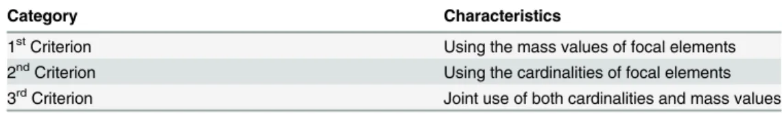
They can also be categorized into three major types depending on the criterion used for removing focal elements as shown inTable 1.
Major available BBA approximations are briefly reviewed below.
Existing BBA Approximations: Type I
The first type of BBA approximation approaches is according to the criterion of the focal ele-ment’s mass assignment, where the focal elements with smaller mass assignments are deemed unimportant, which are first removed. In this type of approaches, there is usually a presetting of the number of remaining focal elementsk. The removal of focal elements is continued until the number of remaining focal elements reachesk.k−l−x[7], Summarization [8] andD1[9]
are representatives for this type.
k
−l−xmethod [7]. This classical approach was proposed by [7], which has three
param-eters. The approximated BBA is obtained by
1. keeping no less thankfocal elements;
2. keeping no more thanlfocal elements;
3. deleting the masses which are no larger thanx.
Ink−l−xapproach, all focal elements in the original BBA are sorted according to their mass
assignments in a decreasing order. Then, the toppfocal elements are selected so thatkpl
and so that the sum of mass assignments of these toppfocal elements is no less than 1−x. The
removed mass assignments are then redistributed to those remaining focal elements by a
Table 1. Categorization of BBA approximations.
Category Characteristics
1stCriterion Using the mass values of focal elements
2ndCriterion Using the cardinalities of focal elements
classical normalization procedure. In fact, ink−l−xmethod, the focal elements with smaller
mass assignments are regarded as“unimportant”ones and thus removed first.
Summarization method [8]. This method also keeps focal elements having largest mass
values as ink−l−xmethod. The mass assignments of removed focal elements are accumulated
and assigned to their union set. Suppose thatmis the original BBA andkis the desired number of remaining focal elements in the approximated BBAmS. LetMdenotes the set ofk−1 focal
elements having the largest mass assignments inm(). ThenmS() is obtained fromm() by
mSðAÞ ¼
mðAÞ; ifA2M
P
A0A;A02=MmðA
0Þ; ifA¼A
0
0; otherwise
ð7Þ
8 > <
> :
whereA0is
A0≜ [
A02=M;mðA0Þ>0A
0 ð8Þ
Note that the number of remaining focal elements could bek(ifA02=M) ork−1 (ifA02 M) after applying Summarization method.
D1 method [9]. Suppose thatmis the original BBA andmSdenotes the approximated
BBA. The desired number of remaining focal elements isk. LetMbe the set ofk−1 focal
ele-ments with the largest mass assignele-ments inmandM−be the set which includes all the other focal elements of the original BBAm. D1 method is to keep all members ofMas the focal ele-ments ofmSand to re-assign the mass assignments of the focal elements inM−among those
focal elements inMaccording to the following procedure.
For a focal elementA2M−, inM, find out all the supersets ofAto construct a collection
MA. IfMAis non-empty,A’s mass assignment is uniformly assigned among those focal
ele-ments having smallest cardinality inMA. WhenMAis empty, then constructMA0 as
MA0 ¼fB2Mjj j B j jA;B\A6¼ ;g ð9Þ
Then, ifM0
Ais non-empty,m(A) is assigned among those focal elements having smallest car-dinality inM0
A. The value assigned to a focal elementBdepends on the cardinality ofB\A, i.e., |
B\A|. The above procedure is iteratively executed until allm(A) have been re-assigned to those focal elements in collectionM.
IfM0
Ais empty, we have two possible cases:
1. If the univeral setΘ2M, the sum of mass assignments of those focal elements inM−will be added toΘ;
2. IfΘ2=M, then letΘbe a focal element ofm
S() and assign the sum of mass assignments of
those focal elements inM−tom
S(Θ).
Note that the number of remaining focal elements isk−1, ifΘ2M. See [9] for more details of
D1 method.
Existing BBA Approximations: Type II
Existing BBA Approximations: Type III
The third type of BBA approximation approaches are based on the criterion of joint using the mass assignments and cardinality of focal elements to determine which focal element should be first removed. Denœux’s inner and outer approximations [11], and our previous works
including the rank-level fusion based approximation [12], and the non-redundancy based BBA approximations [13] belong to this type. In these approaches, the numberkof remaining focal elements is preset.
Denœux’s inner and outer approximations [11]. In Denœux’s inner and outer
approxi-mations, two different distances between focal elements (intersection-basedδ\and union-basedδ[) are used, which are defined as
d[ðA
i;AjÞ ¼ ½mðAiÞ þmðAjÞ jAi[Ajj
mðAiÞ jAij mðAjÞ jAjj
ð10Þ
d
\ðAi;Ajj ¼mðAiÞ jAij þmðAjÞ jAjj
½mðAiÞ þmðAjÞ jAi\Ajj
ð11Þ
Such distances between focal elements consider both the information of the cardinality and mass assignment of the focal element.
“Similar”focal elements defined based onδ\are aggregated by the intersection operation to reduce the number of focal elements, which is called the inner approximation.“Similar”focal elements defined based onδ[are aggregated by the union operation to reduce the number of focal elements, which is called the outer approximation. The focal elements are pairwise aggre-gated till the desired focal elements number is reached. Note that the focal element obtained using aggregation (no matter union or intersection) might be a focal element of the original BBA, therefore, the number of remaining focal elements cannot be estimated precisely. Fur-thermore, inner approximation might bring the empty set;using intersection operation, which is not allowed in the classical“closed-world”DST.
See [11] for more details and illustrative examples.
Rank-level fusion based approximation [12]. In rank-level fusion based approximations,
two ranks of all focal elements in the original BBA are obtained based on each focal element’s cardinality and mass assignment, respectively. Then two ranks are fused to generate a new rank, which can describe both the information of mass assignment and the cardinality. The focal elements with smaller rank position will be removed at first, which represents that they are with smaller mass assignments and with bigger cardinality size at the same time. The proce-dure is briefly introduced below.
1. Sort all the focal elements of an original BBA (withLfocal elements) according to the mass assignment values (in ascending order which is due to the assumption that the focal element with small mass should be deleted as early as possible). The rank vector obtained is
rm¼ ½rmð1Þ;rmð2Þ; :::;rmðLÞ ð12Þ
whererm(i) denotes the rank position of theith focal elements (i= 1,. . .,L) in the original
BBA according to the mass assignment.
deleted as early as possible). The rank vector can be obtained as
rc ¼ ½rcð1Þ;rcð2Þ; :::;rcðLÞ ð13Þ
whererc(i) denotes the rank position of theith focal elements in the original BBA according
to the cardinality.
3. According to the rank-level fusion, we can obtain a fused rank as
rf ¼ ½rfð1Þ;rfð2Þ; :::;rfðLÞ ð14Þ
where
rfðiÞ ¼arfðiÞ þ ð1 aÞ rcðiÞ ð15Þ
andα2[0, 1] is used to show the preference of two different criteria. Such a fused rank can be regarded as a more comprehensive criterion containing both the information of mass assignments and cardinality.
4. Sortffin ascending order and find the focal element with the smallestrfvalue, i.e.,
rfðjÞ ¼min
i rfðiÞ. Then remove thejth focal element in the original BBA.
5. Repeat steps 1) -5) till onlykfocal elements remain. Do re-normalization of the remainingk
focal elements. Finally, output the approximated BBA.
See [12] for more details and illustrative examples.
Non-redundancy based approximations [13]. In non-redundancy based approximations,
the degrees of non-redundancy are defined based on the distances of focal elements as shown inEq (11). First, calculate the distance matrix for all the focal elements ofm() as
MatFE≜
d\ A
1;A1
ð Þ d\ A
1;A2
ð Þ d\ A
1;Al
ð Þ
d
\ðA2;A1Þ d\ðA2;A2Þ d\ðA2;AlÞ
.. . .. . . . . .. . d
\ðAl;A1Þ d\ðAl;A2Þ d\ðAl;AlÞ 2 6 6 6 6 6 4 3 7 7 7 7 7 5
It should be noted thatδ\(Ai,Ai) = 0 andδ\(Ai,Aj) =δ\(Aj,Ai) wherei= 1,. . .,l. Hence, it is not necessary to calculate all the elements inMatFEbecause the matrix is symmetric.
We define the degree of non-redundancy of the focal elementAiby
nRdð ÞAi ≜
1
l 1
Xl 1
j¼1
d \ Ai;Aj
ð16Þ
As we can see that the definitions on degree of redundancy also use both the information of the cardinality and mass assignment of the focal element. The larger nRd(Ai) value, the larger
non-redundancy (less non-redundancy) forAi. The less nRd(Ai) value, the less non-redundancy (larger
redundancy) forAi. Those more redundant focal elements should be removed atfirst. See [13]
for more details and illustrative examples.
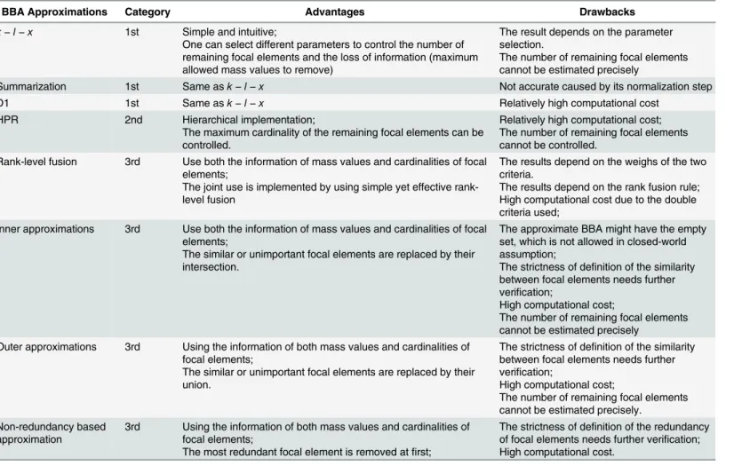
The categorization, pros and cons of the above BBA approximations are illustrated in
Table 2below.
better direction, the current joint use of mass assignments and cardinalities still have some limitations.
For example, in the rank-level based approximation [12], although it is simple, but it is at the price of loss of information due to rank-level fusion when compared with the data-level fusion. Furthermore, there exists the problem of parameter (the weights of mass assignment and cardinality) selection.
In Denœux’s inner and outer approximations [11], the strictness of the distances between
focal elements are not seriously checked till now. Furthermore, when using inner approxima-tion, the empty set;can be generated as a focal element, which is not allowed in the classical DST based on the closed-world assumption.
Also in non-redundancy degree based approximations [13], the rationality and strictness of the definitions on non-redundancy for focal elements still need further inspections.
In summary, the current joint use of mass assignments and cardinalities for the BBA approximation is still an open problem. Therefore, in this paper, we propose another approxi-mation according to the joint use of the mass assignment and the cardinality from a different angle, which is introduced in the next section.
Table 2. Comparisons of different BBA approximations.
BBA Approximations Category Advantages Drawbacks
k−l−x 1st Simple and intuitive;
One can select different parameters to control the number of remaining focal elements and the loss of information (maximum allowed mass values to remove)
The result depends on the parameter selection.
The number of remaining focal elements cannot be estimated precisely
Summarization 1st Same ask−l−x Not accurate caused by its normalization step
D1 1st Same ask
−l−x Relatively high computational cost
HPR 2nd Hierarchical implementation;
The maximum cardinality of the remaining focal elements can be controlled.
Relatively high computational cost; The number of remaining focal elements cannot be controlled.
Rank-level fusion 3rd Use both the information of mass values and cardinalities of focal elements;
The joint use is implemented by using simple yet effective rank-level fusion
The results depend on the weighs of the two criteria.
The results depend on the rank fusion rule; High computational cost due to the double criteria used;
Inner approximations 3rd Use both the information of mass values and cardinalities of focal elements;
The similar or unimportant focal elements are replaced by their intersection.
The approximate BBA might have the empty set, which is not allowed in closed-world assumption;
The strictness of definition of the similarity between focal elements needs further verification;
High computational cost;
The number of remaining focal elements cannot be estimated precisely
Outer approximations 3rd Using the information of both mass values and cardinalities of focal elements;
The similar or unimportant focal elements are replaced by their union.
The strictness of definition of the similarity between focal elements needs further verification;
High computational cost;
The number of remaining focal elements cannot be estimated precisely.
Non-redundancy based
approximation 3rd Using the information of both mass values and cardinalities offocal elements; The most redundant focal element is removed atfirst;
The strictness of definition of the redundancy of focal elements needs further verification; High computational cost.
A Novel BBA Approximation Using Distance of Evidence
To be more direct and to use more information, in this paper, we start from the performance evaluation of BBA approximations for designing new BBA approximation approaches. The basic idea is as follows.
In the available related literatures, the performance evaluation of BBA approximations often includes the evaluation in terms of the computational cost and the evaluation in terms of the information loss.
Intuitively, a better BBA approximation should output a BBA having less computational cost for the operations in DST, e.g., the evidence combination, and being more similar to the original BBA (less loss of information). The similarity can be described using the distance of evidence inEq (5). So far as we remove some focal elements, the computational cost will be decreased more or less. Here, we focus on the closeness between the approximated BBA and the original one.
In all possible approximated BBAs, the one having smaller distance from the original one is preferred. If one want to obtain such a BBA denoted bymopt, one can pick the one minimizing
the chosen distance with respect to the original BBA among all the possible BBAs havingk
focal elements according to
mopt ¼ms
s¼arg i
mindJðmi;mÞ
s:t:
i¼1; :::L
the number of focal elements in mi is k
ð17Þ
(
However, such an optimal way is time-consuming and might cause the BBA approximation intractable, especially when the number of focal elements is very large (we provide a detailed analysis on this at the end of this section). Therefore, we try to make a trade-off between the optimality and the tractability by introducing an iterative implementation. We design an itera-tive BBA approximation approach based on minimizing the distance of evidence between the approximated BBA in current iteration and the BBA obtained in the previous iteration.
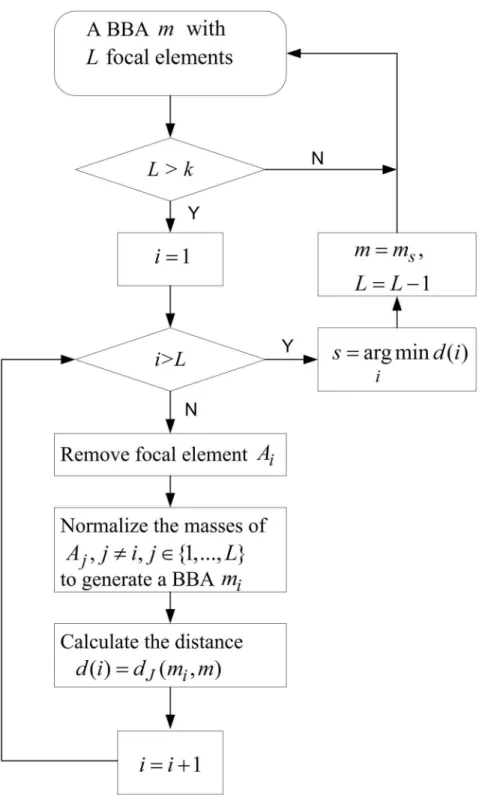
Given a BBAmwithLfocal elementsA1,. . .,AL. Suppose that the desired number of
remaining focal elements isk. The specific implementation is as follows.
Step 1:Remove a focal elementAifromm. Normalize the mass of the remainingAj, wherej6¼ iandj2{1,. . .,L}, to generate a new BBAm0i.
Step 2:Calculate the distance betweenm0iandmdenoted byd(i). Execute Step 1 and Step 2 for alli= 1,. . .,L.
Step 3:Find the minimum values ofd(i),i= 1,. . .,L, i.e.,
s¼arg
i
mindðiÞ
Step 4:Remove the focal elementAsfrommand de the normalization to generate an
approxi-mated BBAms. Such a new BBAmsis closest to the BBAmcompared with those obtained
by removing any other focal elementAj, wherej6¼s,j2{1,. . .,L}. Reduce the number of
focal elements by one, i.e.,L=L−1.
Step 5:Assignm=ms. If the desired number of remaining focal elements is not reached, i.e.,L
The whole procedure is illustrated inFig 1.
Here we provide an illustrative example to show how the BBA approximation using distance of evidence works.
Fig 1. Procedure of the iterative BBA approximation using distance of evidence.Illustration of the whole procedure of the new iterative approximation.
Example 1
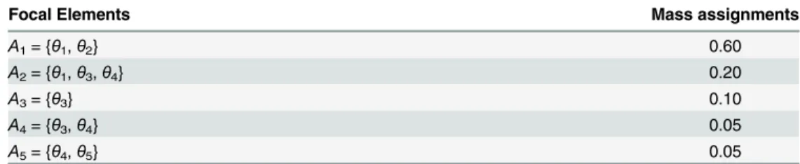
Let’s consider the BBAm() defined over the FODΘ= {θ1,θ2,θ3,θ4,θ5} listed inTable 3.
Here the numberkof the remaining focal elements is set to 3. Now, we apply the iteration BBA approximation based on distance of evidence tom.
In the first iteration, when we removeA1= {θ1,θ2}, the BBA obtained is as follows.
m1ðA2Þ ¼0:5000;m1ðA3Þ ¼0:2500;m1ðA4Þ ¼0:1250;m1ðA5Þ ¼0:1250:
The corresponding distance of evidencedJ(m1,m) = 0.4899
When we removeA2= {θ1,θ3,θ4}, the BBA obtained is
m2ðA1Þ ¼0:7500;m2ðA3Þ ¼0:1250;m2ðA4Þ ¼0:0625;m2ðA5Þ ¼0:6250:
anddJ(m2,m) = 0.1431.
When we removeA3= {θ3}, the BBA obtained is
m3ðA1Þ ¼0:6667;m3ðA2Þ ¼0:2222;m3ðA4Þ ¼0:0556;m3ðA5Þ ¼0:0556:
anddJ(m3,m) = 0.0835
When we removeA4= {θ3,θ4}, the BBA obtained is
m4ðA1Þ ¼0:6316;m4ðA2Þ ¼0:2105;m4ðA3Þ ¼0:1053;m4ðA5Þ ¼0:0526:
anddJ(m4,m) = 0.0375
When we removeA5= {θ4,θ5}, the BBA obtained is
m5ðA1Þ ¼0:6316;m5ðA2Þ ¼0:2105;m5ðA3Þ ¼0:1053;m5ðA4Þ ¼0:0526:
anddJ(m5,m) = 0.0421.
dJ(m4,m) is the smallest, therefore, the focal element removed in 1st iteration isA4. After
the 1st iteration, the number of focal elements is 4.
Then, in the second iteration, the BBA to approximate ismm m4, i.e.,
mmðB1Þ ¼0:6316;mmðB2Þ ¼0:2105;mmðB3Þ ¼0:1053;mmðB4Þ ¼0:0526:
whereB1=A1,B2=A2,B3=A3,B4=A5.
When we removeB1= {θ1,θ2}, the BBA obtained is
mm1ðB2Þ ¼0:5714;mm1ðB3Þ ¼0:2857;mm1ðB4Þ ¼0:1429:
anddJ(mm1,mm) = 0.5077.
When we removeB2= {θ1,θ3,θ4}, the BBA obtained is
mm2ðB1Þ ¼0:8000;mm2ðB3Þ ¼0:1333;mm2ðB4Þ ¼0:0667:
anddJ(mm2,mm) = 0.1589.
Table 3. Focal elements and mass values ofm().
Focal Elements Mass assignments
A1= {θ1,θ2} 0.60
A2= {θ1,θ3,θ4} 0.20
A3= {θ3} 0.10
A4= {θ3,θ4} 0.05
A5= {θ4,θ5} 0.05
When we removeB3= {θ3}, the BBA obtained is
mm3ðB1Þ ¼0:7059;mm3ðB2Þ ¼0:2353;mm3ðB4Þ ¼0:0588:
anddJ(mm3,mm) = 0.0909.
When we removeB4= {θ4,θ5}, the BBA obtained is
mm4ðB1Þ ¼0:6667;mm4ðB2Þ ¼0:2222;mm4ðB3Þ ¼0:1111:
anddJ(mm4,mm) = 0.0454.
dJ(mm4,mm) is the smallest, therefore, the focal element removed in 2nd iteration isB4, i.e., A5. After the 2nd iteration, the number of focal elements reaches 3 and then the iteration stops.
The final output approximated BBA ismo mm4.
Here, we also provide the approximation results of the available BBA approximations referred in the previous section for comparisons.
Usingk−l−xmethod [7]. Herekandlare set to 3.xis set to 0.1. The focal elementsA4
= {θ3,θ4} andA5= {θ4,θ5} are removed without violating the constraints ink−l−x. The
remaining total mass value is 1−0.05−0.05 = 0.9. Then, all the remaining focal elements’
mass values are divided by 0.9 to accomplish the normalization. The approximated BBA
mklx
S ðÞobtained byk−l−xmethod is listed inTable 4, whereA0i,i= 1, 2, 3 are the focal ele-ments ofmklx
S ðÞ.
Using summarization method [8]. Herekis set to 3. According to the summarization
method, the focal elementsA3= {θ3},A4= {θ3,θ4} andA5= {θ4,θ5} are removed, and their
union {θ3,θ4,θ5} is generated as a new focal element with mass valuem({θ3}) +m({θ3,θ4}) +m
({θ4,θ5}) = 0.2. The approximated BBAmSum
S is listed inTable 5below.
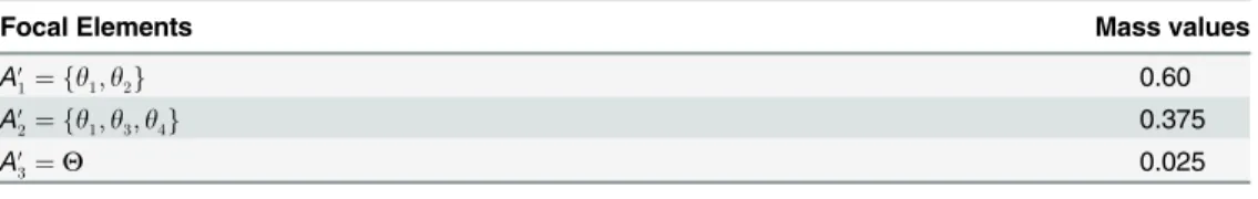
Using D1 method [9]. Herekis still 3. It can be obtained thatA1,A2belong toM, andA3, A4,A5belong toM−. The focal elementA1= {θ1,θ2} has empty intersection with the focal
ele-ments inM−, therefore its value will be unchanged. InM,A
2is the unique superset ofA3and A4, therefore,m(A3) +m(A4) = 0.10 + 0.05 is added to its original mass value.A2also covers
half ofA5, therefore,m(A5)/2 = 0.025 is further added to the mass ofA2. Finally, the rest mass
value is assigned to the total setΘ. The approximated BBAmD1
S is listed inTable 6.
Using Rank-level fusion based approximation [12]. The number of remaining focal
ele-ments is 3. The approximate BBA is as shown inTable 7. It should be noted that although for Example 1,mRank
S ðÞ ¼m klx
S ðÞ, they are two different approaches. Table 4.mklx
SðÞobtained usingk−l−x.
Focal Elements Mass values
A0
1¼ fy1;y2g 0.6667
A0
2¼ fy1;y3;y4g 0.2222
A0
3¼ fy3g 0.1111
doi:10.1371/journal.pone.0147799.t004
Table 5.mSum
S ðÞobtained using Summarization.
Focal Elements Mass values
A0
1¼ fy1;y2g 0.60
A0
2¼ fy1;y3;y4g 0.20
A0
3¼ fy3;y4;y5g 0.20
Using Denœux inner and outer approximation [11]. With the inner approximation
method, the focal elements pair with smallest Denouex’s inner distance are removed, and then their intersection is set as the supplemented focal element whose mass value is the sum of the removed two focal elements’mass values. Such a procedure is repeated until the desired num-ber of focal elements is reached. The results at each step are listed inTable 8.
As we can see inTable 8, it generates the empty set as a focal element, which is not allowed in the classical Dempster-Shafer evidence theory under close-world assumption.
With the outer approximation method, the focal elements pair with smallest Denouex’s outer distance are removed, and then their union is set as the supplemented focal element whose mass value is the sum of the removed two focal elements’mass values. Such a procedure is repeated until the desired number of focal elements is reached. The results at each step are listed inTable 9.
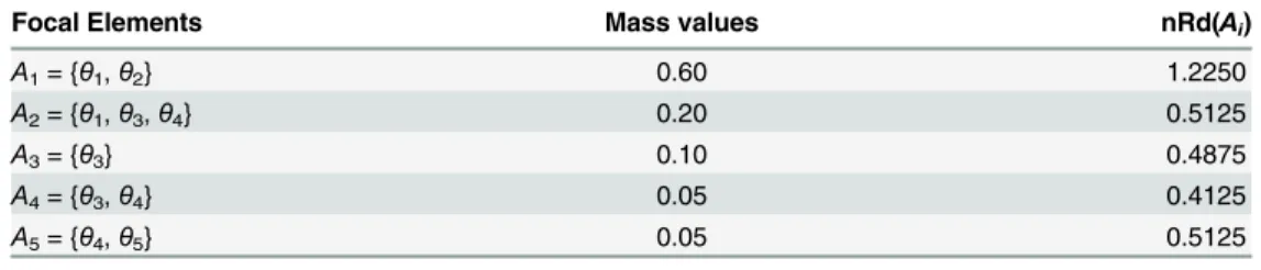
Using the redundancy-based batch approximation method [13]. The desired remaining
focal element is set tok= 3. We first calculate the distance matrixMatFE, based on which, the
degree of non-redundancy for each focal elements ofm() can be obtained. It is listed in
Table 10.
SinceA3andA4at the bottom have the two least nRd values, they correspond the two focal
elements with the lowest non-redundancy, i.e., the highest redundancy. Therefore, they are Table 6.mD1
SðÞobtained using D1.
Focal Elements Mass values
A0
1¼ fy1;y2g 0.60
A0
2¼ fy1;y3;y4g 0.375
A0
3¼Y 0.025
doi:10.1371/journal.pone.0147799.t006
Table 7.mRank
S ðÞobtained using Rank-level fusion.
Focal Elements Mass values
A0
1¼ fy1;y2g 0.6667
A0
2¼ fy1;y3;y4g 0.2222
A0
3¼ fy3g 0.1111
doi:10.1371/journal.pone.0147799.t007
Table 8.mRank
S ðÞobtained using inner approximation.
Focal Elements Mass values
A0
1¼ fy1;y2g 0.6000
A0
2¼ fy1;y3;y4g 0.2000
A0
3¼ ; 0.1111
doi:10.1371/journal.pone.0147799.t008
Table 9.mRank
S ðÞobtained using outer approximation.
Focal Elements Mass values
A0
1¼ fy1;y2g 0.6000
A0
2¼ fy1;y3;y4g 0.3500
A0
3¼ fy4;y5g 0.0500
removed and their mass values are redistributed thanks to the classical normalization step. The approximated BBAmBRd
S is listed inTable 11.
Further discussion on the iterative approximation based on distance of
evidence
As aforementioned, the BBA obtained using the above iterative approximation is usually not the BBA which is closest to the original BBA given a desired numberkof remaining focal ele-ments, however it can significantly reduce the computational cost caused by the optimization, thus, is more tractable. It can also obtain relative smaller distance when compared with other BBA approximations as verified in the experiment below.
If we are too greedy for obtaining the minimum distance, the price is the significantly increased computational cost in BBA approximation. Given the number of remaining focal ele-mentsk, there are totallyCk
2n 1different BBAs. The approximated BBA with minimum distance to the original one should be selected out of theCk
ndifferent BBAs. Using our iterative approxi-mation, there are totally
C1
2n 1þC12n 1 1þ þC1kþ1
¼C1
2n 1þC12n 1 1þ þC21n 1 ð2n 1 ðkþ1ÞÞ
¼2n 1þ2n 1 1þ þ2n 1 ð2n 1 ðkþ1ÞÞ
¼ ð2n 1 kÞ ð2n 1Þ ð2
n 1 kÞð2n 1 k 1Þ
2 ¼2n 2n 1þk=2
BBAs. When the |Θ| = 5, the size of searching space for the onefinding the minimum one and
our iterative approximation are compared at differentkas shown inTable 12.
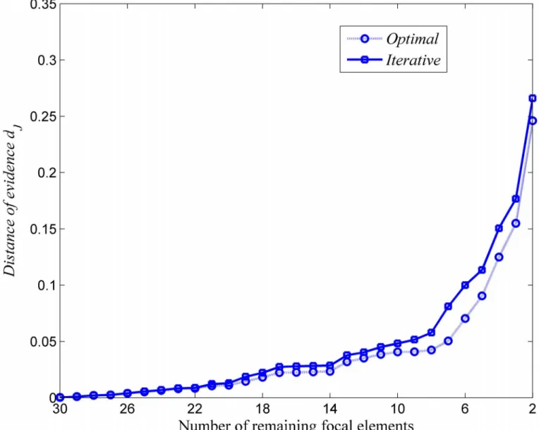
The distance of evidence between the approximated BBA and the original one for the one finding the minimum one and our iterative approximation are compared at differentkas shown inFig 2.
As shown inFig 2andTable 12, the approach to finding the minimum distance does pro-vide the minimum loss of information, however, it is at the price of extremely large computa-tional cost for the approximation, which makes the approximation intractable, especially when Table 10. Non-redundancy for different focal elements.
Focal Elements Mass values nRd(Ai)
A1= {θ1,θ2} 0.60 1.2250
A2= {θ1,θ3,θ4} 0.20 0.5125
A3= {θ3} 0.10 0.4875
A4= {θ3,θ4} 0.05 0.4125
A5= {θ4,θ5} 0.05 0.5125
doi:10.1371/journal.pone.0147799.t010
Table 11.mBRd
S ðÞobtained using the batch approximation based on redundancy.
Focal Elements Mass values
A0
1¼ fy1;y2g 0.7059
A0
2¼ fy1;y3;y4g 0.2353
A0
3¼ fy4;y5g 0.0588
the |Θ| is very large. Our new proposed iterative approximation can make a good trade-off
between the precision (with less loss of information) and the tractability (without so large computational cost).
To well justify our newly proposed BBA approximation, we give more detailed analyses on the evaluation of BBA approximations at first in the next section.
Further analyses on evaluations of BBA approximations
Evaluation criteria of BBA approximations
The evaluation criteria are very crucial for evaluate different BBA approximations, and also for design new BBA approximations. The available BBA approximation evaluation approaches are as follows.
1) Reduction of the computational cost after approximation
After the BBA approximation, the computational operations like evidence combination, conditioning, marginalization, belief and plausibility degrees evaluation will be reduced. The BBA approximation with larger degree of reduction is preferred.
2) Closeness between the approximated BBA and the original one
Table 12. Size of searching space.
Number of Remaining FEs Optimal Iterative
30 31 31
29 465 61
28 4495 90
27 31465 118
26 169911 145
25 736281 171
24 2629575 196
23 7888725 220
22 20160075 243
21 44352165 265
20 84672315 286
19 141120525 306
18 206253075 325
17 265182525 343
16 300540195 360
15 300540195 376
14 265182525 391
13 206253075 405
12 141120525 418
11 84672315 430
10 44352165 441
9 20160075 451
8 7888725 460
7 2629575 468
6 736281 475
5 169911 481
4 31465 486
3 4495 490
2 465 493
After the BBA approximation, the BBA obtainedm0will depart from the original one. Larger degree of such a departure, i.e., less closeness between the approximated BBAm0and the original onem, means larger loss of information, which is not preferred. Such a degree of departure (or degree of closeness) can be described using the distance of evidence defined in
Eq (5), i.e.,dJ(m,m0).
3) Degree of ordering preservation between plausibilities of events
In a BBA, each focal element corresponds to an event. Based on a given BBAm, we can cal-culate the corresponding plausibility functionPlaccording toEq (2). Then, the ordering or ranking of the plausibilitiesPl(Ai),Ai22
Θ
of different focal elements (events) can be obtained, which is noted byΛ
Pl. After the BBA approximation, we obtain the approximated BBAm0and
can calculate its plausibilitiesPl0(Bi),Bi22
Θ
and its ordering denoted byΛPl0. We can calculate
Fig 2. Comparisons on closeness for the optimal and the iterative approaches.Evaluation in terms of the loss of information for the optimal and iterative ways.
the distance betweenΛPlandΛPl0using Spearman’s distance [21]:
dPl¼1
LPl LPl
L
Pl0 LPl0
T
ffiffiffiffiffiffiffiffiffiffiffiffiffiffiffiffiffiffiffiffiffiffiffiffiffiffiffiffiffiffiffiffiffiffiffiffiffiffiffiffiffiffiffiffiffiffiffiffiffiffiffi
LPl LPl
L
Pl LPl
T
q
ffiffiffiffiffiffiffiffiffiffiffiffiffiffiffiffiffiffiffiffiffiffiffiffiffiffiffiffiffiffiffiffiffiffiffiffiffiffiffiffiffiffiffiffiffiffiffiffiffiffiffiffiffiffi
LPl0 LPl0
L
Pl0 LPl0
T
q ð18Þ
where smaller distance representing less loss of information or less distortion brought by the approximation is preferred.
4) Preservation of inclusion relation
Suppose that two BBAsm1andm2satisfy the inclusion relation (e.g.,s-inclusion), which is
defined as follows [22].
Suppose thatm1’s focal elements are {A1,. . .,Aq} andm2’s focal elements are {B1,. . .,Bp}. If
and only if there exists a non-negative matrixG= [gi,j] such that forj= 1,. . .,p,
Pq
i¼1gij¼1;gij>0)AiBj, and fori= 1,. . .,q, Pp
j¼1m2ðBjÞgi;j¼1, wheregijis the
pro-portion ofBjthat“flows down”toAi. That is,m1iss-included inm2(m1vsm2) if the mass of
any focal elementBjofm2can be redistributed among subsets ofBjinm1. This means thatm1
is less informative thanm2.
After the approximation, if their approximated BBAsm0
1andm
0
2still satisfy the inclusion relation, such a BBA approximation is preferred. This represents the informative relation between two BBAs is not affected by the approximation.
It should be noted that preservation of inclusion relation is a very strict relation. We have checked that all the BBA approximations introduced in this paper including our new approach cannot satisfy it.
Besides the above criteria, in this paper, we propose two new evaluation criteria for BBA approximations as follows.
New criterion I: Order preservation in terms of uncertainty degrees
Giventdifferent BBAs (according to Algorithm 1 [23] inTable 2):m1,. . .,mtand calculate
their corresponding degree of uncertainty, e.g., the aggregated uncertainty (AU) [24,25] as defined below.
AUðmÞ ¼max Pm ½
X
y2Y
pylog2py ð19Þ
where the maximum is taken over all probability distributions being consistent with the given BBA.Pmconsists of all probability distributionshpθ|θ2Θisatisfying:
py 2 ½0;1;8y2Y
P
y2Ypy ¼1
BelðAÞ P
y2Apy1 BelðAÞ; 8AY
ð20Þ
8 > <
> :
For thetBBAs, their corresponding AU values areAU(m1),. . .,AU(mt). Then, sort AU values
in an ascending order to obtain a rankingΛ
o. Apply a BBA approximation approachSito all the tBBAs, thentapproximated BBAs can be obtained asmi
1; :::;m i
t. Calculate and sort the AU val-ues also in an ascending order to obtain a rankingΛi. Calculate the distance betweenΛoandΛi.
If two rankings before and after the approximationSiare closer to each other, thenSiis
Here, we can use the Spearman’s distance [21] to measure the rankings’difference as fol-lows.
do;i ¼1
Lo Lo
L
i Li
T
ffiffiffiffiffiffiffiffiffiffiffiffiffiffiffiffiffiffiffiffiffiffiffiffiffiffiffiffiffiffiffiffiffiffiffiffiffiffiffiffiffiffiffiffiffi
Lo Lo
L
o Lo
T
q
ffiffiffiffiffiffiffiffiffiffiffiffiffiffiffiffiffiffiffiffiffiffiffiffiffiffiffiffiffiffiffiffiffiffiffiffiffiffiffiffiffiffi
Li Li
L
i Li
T
q ð21Þ
New criterion II: Preservation of probabilistic decision
After we apply the Pignisitc Probability Transformation (PPT) [26] to a BBAmaccording to
BetPðy
iÞ ¼ X
yi2B; B22Y
mðBÞ
jBj ; ð22Þ
the decision can be made by selecting theθiwith the maximum value in BetP(θj),j= 1,. . ., |Θ|.
If the probabilistic decision for the approximated BBAm0(usingSi) is the same as the
prob-abilistic decision obtained based on the original BBAm, then the approximationSiis desired.
Such a criterion describes the probabilistic decision consistency before and after the BBA approximation.
One can use Monte Carlo method based on all the above criteria to evaluate BBA approxi-mations. See details of implementation in the simulations in the next section.
Experiments and Simulations
In this section, we compare all the BBA approximation approaches aforementioned with the preset of remaining focal elements’numberkincludingk−l−x(denoted byS1),
Summariza-tion (S2), D1 (S3), rank-level fusion based approximation (S4), the non-redundancy based
approximation (S5), and Denœux’s outer approximations (S6) (we do not compare inner
approximation method which might bring troubles for making the comparisons because Jous-selme’s distance cannot be computed if one allows to assign positive mass on empty set due to |;| = 0), with our newly proposed BBA approximation approach (S7).
Simulation I—Comparisons in terms of computational time and the closeness. In
Sim-ulation I, we use the computational time of the evidence combination and the distance of evi-dence between the approximated BBA and the original one in average as performance measures. Our comparative analysis is based on a Monte Carlo simulation usingM= 200 ran-dom runs. The size of the FOD is |Θ| = 6. In thejth simulation run, a BBAmj() is randomly
generated according to Algorithm 1 [23] inTable 13. In each random generation, there are 26
−1 = 63 focal elements in the BBAmj() to approximate. The number of remaining focal
ele-mentskfor all the approaches used here are set to from 62 to 2. Then, different approximation
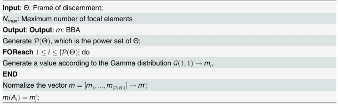
Table 13. Algorithm 1: Random BBA generation—Uniform sampling from all focal elements.
Input:Θ: Frame of discernment; Nmax: Maximum number of focal elements Output:Output:m: BBA
GeneratePðYÞ, which is the power set ofΘ;
FOReach1i jPðYÞjdo
Generate a value according to the Gamma distributionGð1;1Þ !mi,
END
Normalize the vectorm¼ ½m
1; :::;mjPðYÞj !m0;
mðAiÞ ¼m0
i;
resultsfmji;kðÞgin thejth run can be obtained using the different approximationSi(i
repre-sents theith BBA approximation approach applied) given different remaining number (k) of focal elements. We record the computational time of the original evidence combination of
mj()mj() with Dempster’s rule of combination, and the computation time of using the Dempster’s rule of combination for each approximated BBAmji;kðÞ m
j
i;kðÞ. The average (over 200 runs) computation time for the original combination and the combination after the approximation are shown inFig 3. The average (over 200 runs) distance values (dJ) between
the original BBA and the approximated BBA’s obtained using different approaches given dif-ferent remaining focal elements’number (k) are shown inFig 4.
As we can see, when compared with the original computational time, the computation time of all the BBA approximation approaches can be reduced. This is intuitive, because the number Fig 3. Computation time comparisons.Evaluation in terms of computational cost.
of focal elements are reduced. At the same time, our newly proposed approximation usually has the smallest distance of evidence, i.e., the largest closeness, which represents the least loss of information when compared with other approximations concerned here.
Simulation II—Comparisons in terms of order-preservation for uncertainty degree. In
Simulation II, we compare the information preservation capability of different BBA approxi-mations from another aspect. Suppose that the size of FOD is 5.
1. Randomly generate 5 different BBAs (according to Algorithm 1 inTable 2):m1,. . .,m5and
calculate their corresponding AUAU(m1),. . .,AU(m5).
2. Sort AU values in an ascending order to obtain a rankΛ
o.
3. Apply a BBA approximation approachSito all the five BBAs, then five approximated BBAs
can be obtained asmi 1; :::;mi5.
Fig 4. Closeness comparisons.Evaluation in terms of the loss of information.
4. Calculate and sort the AU values also in an ascending order to obtain a rankΛ
i.
5. Calculate the distance betweenΛoandΛi.
If two rankings before and after the approximationSiare closer to each other, thenSiis
pre-ferred for such an capability of order preservation, which represents a less loss of information from another aspect.
The above simulation procedure is repeated 500 times (in each run, 5 BBAs are re-generated randomly), the different approximationSi’s averaged distances of ordering at differentkare
listed inFig 5.
The average distance of ordering over allkfor different approximations are listed inTable 14. Fig 5. Comparisons in terms of order-preservation for uncertainty.Evaluation of distortion caused by the approximation in terms of uncertainty degree.
As we can see in theFig 5andTable 14that our newly proposed approach usually has the smallest average distance between two orderings, which represents the high capability in order-preservation, i.e., our new approach only causes the relatively small change to the order of the uncertainty degree. As aforementioned, this also represents the less loss of information and less distortion of relation caused by the approximation.
Simulation III—Comparisons in terms of probabilistic decision preservation. In this
Simulation III, we compare all the BBA approximations in terms of the probabilistic decision preservation. It is hard to make the decision based on the original BBA and the decision based on the approximated one always have the same results, therefore, we calculate the percentage of the probabilistic preservation forSias follows.
1. Randomly generate 1000 BBAs. One can also select 1000 BBAs out of the 10000 generated BBAs in the data set (S1 File).
2. Make probabilistic decision for the 1000 different original BBAs.
3. Apply the BBA approximationSito the 1000 original BBAs.
4. Make probabilistic decision for the 1000 different approximated BBAs.
5. Count the numberNiof cases where the probabilistic decision results for the original BBA and its corresponding approximated BBA usingSiare the same.
6. Output the percentagePd(i) =Ni/1000 × 100%.
The random generation of BBAs is according to Algorithm 1 inTable 13. A BBA approxi-mationSiwith higherPd(i) is more preferred. In this simulation, the FODΘis with cardinality
of 5. The simulation results (i.e., the percentage of probabilistic decision preservation for vari-ous BBA approximations with preset different remaining focal elements’numberk) are shown inFig 6.
The average consistency rate over allkfor different approximations are listed inTable 15. As we can see inFig 6andTable 15that the percentage of the probabilistic decision results preservation of the rank-level fusion based approximation and our newly proposed approach is usually highest (or the 2nd highest). It means that our new approach has higher possibility to keep the probabilistic decision results before and after the approximation unchanged given preset number of remaining focal elements, which represents the less loss of information from a different angle and the less of distortion of the relation caused by the approximation.
Simulation IV—Comparisons in terms of plausibility preservation. In this simulation
IV, we compare all the BBA approximations in terms of the probabilistic decision preservation.
1. Randomly generate 1000 BBAs according to Algorithm 1. Table 14. Averaged distance of ordering over allkvalues.
BBA approximations Distance of ordering
S1 0.1679
S2 0.1576
S3 0.1874
S4 0.1667
S5 0.1808
S6 0.1698
S7 0.1513
2. For each BBAmj,j= 1,. . ., 1000, calculate its corresponding plausibilities and generate the
orderingLi
Pl.
3. After applying a BBA approximationSi, calculate the corresponding plausibilities and
gen-erate the orderingLj
Pl0.
4. Calculate the distance betweenLj
PlandL j
Pl0denoted bydji,j= 1,. . ., 1000.
5. Output the average distancedi¼P1000j¼1 d j i=1000.
Fig 6. Comparisons in terms of probabilistic decision consistency.Evaluation of the distortion in terms of the probabilistic decision.
TheSiwith smallerdivalue is more preferred.
The average distance of ordering over allkfor different approximations are listed in
Table 16. the different approximationSi’s averaged distances of ordering at differentkare listed
inFig 7.
As we can see in theFig 7andTable 16that the rank-level fusion based approximation and our newly proposed approach usually has the smallest average distance between two orderings, which represents the high capability in order-preservation for the plausibilities, i.e., our new approach only causes the relatively small change to the order of the plausibilities of events. It represents the less distortion caused by the BBA approximation.
Conclusions
A novel iterative BBA approximation approach based on the distance of evidence and two new evaluation approaches for BBA approximations are proposed in this paper. The new approxi-mation can effectively simplify the BBA, and is with less loss of inforapproxi-mation. It also makes a good balance between the precision and the tractability of the approximation. Two new perfor-mance evaluation approaches for BBA approximations are related to the uncertainty order-preservation and the consistency of probabilistic decision, respectively. Simulations and experi-ments are provided to illustrate and support our new BBA approximation and related evalua-tion approaches.
In this paper, we use the distance of evidence (closeness) to measure the loss of information in the BBA approximation. The closeness between two BBAs has strong correlation with the difference of information in two BBAs, thus, the closeness can be used to represent the loss of information. However, to be more strict, they are two different concepts. In our future work, we will try to directly use the difference between the degrees of uncertainty for BBAs (not the difference between the orders of uncertainty degree as we proposed in the uncertainty Table 15. Averaged probabilistic decision consistency rate over allkvalues.
BBA approximations Distance of ordering
S1 0.8626
S2 0.8432
S3 0.8396
S4 0.8773
S5 0.8271
S6 0.8039
S7 0.8732
doi:10.1371/journal.pone.0147799.t015
Table 16. Averaged distance of ordering over allkvalues.
BBA approximations Distance of ordering
S1 0.0318
S2 0.0390
S3 0.0366
S4 0.0240
S5 0.0371
S6 0.0409
S7 0.0256
preservation) to represent the loss of information. The problem is how to design or select com-prehensive uncertainty measures for BBAs, because the current total uncertainty measures in evidence theory including AU used in this paper and the ambiguity measure (AM) [27] are designed by generalizing the uncertainty measures in the probabilistic framework. They all have limitations [27,28] and cannot always comprehensively describe the uncertainty in a BBA. Furthermore, although we propose two evaluation approaches for BBA approximations, how to evaluate the BBA approximation is still an opening and challenging problem. More solid, especially quantitative performance evaluation approaches are our research focus in future.
Fig 7. Comparisons in terms of order-preservation for plausibilities.Evaluation of the distortion caused by the approximation in terms of plausibilities.
Supporting Information
S1 File. 10000 BBAs for test.Totally 10000 different BBAs for testing different approximation
approach. (MAT)
Acknowledgments
The authors thank the reviewers and editors for giving valuable comments, which are very helpful for improving this manuscript.
Author Contributions
Conceived and designed the experiments: YY. Performed the experiments: YY YL. Analyzed the data: YY YL. Contributed reagents/materials/analysis tools: YY. Wrote the paper: YY YL.
References
1. Shafer G, et al. A mathematical theory of evidence. vol. 1. Princeton university press Princeton; 1976. 2. Laamari Wafa, Ben Yaghlane Boutheina. Propagation of Belief Functions in Singly-Connected Hybrid
Directed Evidential Networks. Scalable Uncertainty Management (Editors: Christoph Beierle and Alex Dekhtyar), vol. 9310. Springer International Publishing; 2015, p. 234–248.
3. Shah Harsheel R. Investigation of robust optimization and evidence theory with stochastic expansions for aerospace. Doctoral Dissertation, Missouri University of Science and Technology, 2015.
4. Smarandache F, Dezert J. Advances and applications of DSmT for information fusion-Collected works-Volume 4. American Research Press; 2015.
5. Smarandache F, Dezert J. Advances and applications of DSmT for information fusion-Collected works-Volume 3. American Research Press; 2009.
6. Smets P. Practical uses of belief functions. In: Proceedings of the Fifteenth conference on Uncertainty in artificial intelligence. Morgan Kaufmann Publishers Inc.; 1999. p. 612–621.
7. Tessem B, et al. Approximations for efficient computation in the theory of evidence. Artificial Intelli-gence. 1993; 61(2):315–329. doi:10.1016/0004-3702(93)90072-J
8. Lowrance JD, Garvey TD, Strat TM. A framework for evidential-reasoning systems. In: Classic Works of the Dempster-Shafer Theory of Belief Functions. Springer; 2008. p. 419–434.
9. Bauer M. Approximations for decision making in the Dempster-Shafer theory of evidence. In: Proceed-ings of the Twelfth international conference on Uncertainty in artificial intelligence. Morgan Kaufmann Publishers Inc.; 1996. p. 73–80.
10. Grabisch M. Upper approximation of non-additive measures by k-additive measures—the case of belief functions. In: ISIPTA; 1999. p. 158–164.
11. Denœux T. Inner and outer approximation of belief structures using a hierarchical clustering approach.
International Journal of Uncertainty, Fuzziness and Knowledge-Based Systems. 2001; 9(04):437–460. doi:10.1142/S0218488501000880
12. Yang Y, Han D, Han C, Cao F. A novel approximation of basic probability assignment based on rank-level fusion. Chinese Journal of Aeronautics. 2013; 26(4):993–999. doi:10.1016/j.cja.2013.04.061 13. Han D, Yang Y, Dezert J. Two novel methods for BBA approximation based on focal element
redun-dancy. In: Proceedings of the 18th International Conference on Information Fusion. ISIF. Washington DC: IEEE; 2015. p. 428–434.
14. Jousselme AL, Grenier D, Bossé É. A new distance between two bodies of evidence. Information fusion. 2001; 2(2):91–101. doi:10.1016/S1566-2535(01)00026-4
15. Bouchard M, Jousselme AL, Doré PE. A proof for the positive definiteness of the Jaccard index matrix. International Journal of Approximate Reasoning. 2013; 54(5):615–626. doi:10.1016/j.ijar.2013.01.006 16. Kennes R. Computational aspects of the Mobius transformation of graphs. Systems, Man and
Cyber-netics, IEEE Transactions on. 1992; 22(2):201–223. doi:10.1109/21.148425
17. Barnett JA. Computational methods for a mathematical theory of evidence. In: Classic Works of the Dempster-Shafer Theory of Belief Functions. Springer; 2008. p. 197–216.
19. Burger T. Defining new approximations of belief functions by means of Dempster’s combination. In: Proc. of the 1st International Workshop on the Theories of Belief Functions (BELIEF 2010), Brest, France, April 1st-April 2nd; 2010.
20. Dezert J, Han D, Liu Z, Tacnet JM. Hierarchical proportional redistribution for bba approximation. In: Belief functions: theory and applications. Springer; 2012. p. 275–283.
21. Myers JL, Well A, Lorch RF. Research design and statistical analysis. Routledge; 2010.
22. Destercke Sébastien, Burger Thomas. Revisiting the notion of conflicting belief functions. Proceedings of the 2nd International Conference on Belief functions. Compiégne, France, May 2012, 153–160. 23. Burger Thomas, Destercke Sébastien. Random generation of mass functions: A short Howto.
Proceed-ings of the 2nd International Conference on Belief functions. Compiégne, France, May 2012, 145–152. 24. Harmanec D, Klir GJ. Measuring total uncertainty in Dempster-Shafer theory: A novel approach.
Inter-national journal of general system. 1994; 22(4):405–419. doi:10.1080/03081079408935225
25. Abellán J, Masegosa A. Requirements for total uncertainty measures in Dempster–Shafer theory of evi-dence. International journal of general systems. 2008; 37(6):733–747. doi:10.1080/
03081070802082486
26. Smets P, Kennes R. The transferable belief model. Artificial intelligence. 1994; 66(2):191–234. doi:10. 1016/0004-3702(94)90026-4
27. Jousselme A -L, Liu C S, Grenier D, Bossé É. Measuring ambiguity in the evidence theory. IEEE Trans-actions on Systems, Man and Cybernetics, Part A: Systems and Humans, 2006; 36(5):890–903. doi: 10.1109/TSMCA.2005.853483