Recovery Trends between 2001 and 2010
Ana Marı´a Sa´nchez-Cuervo1*, T. Mitchell Aide1, Matthew L. Clark2, Andre´s Etter3
1Department of Biology, University of Puerto Rico, San Juan, Puerto Rico, United States of America,2Department of Geography and Global Studies, Sonoma State University, Rohnert Park, California, United States of America,3Departamento de Ecologı´a y Territorio, Universidad Javeriana, Bogota´ D.C., Colombia
Abstract
Background:Monitoring land change at multiple spatial scales is essential for identifying hotspots of change, and for developing and implementing policies for conserving biodiversity and habitats. In the high diversity country of Colombia, these types of analyses are difficult because there is no consistent wall-to-wall, multi-temporal dataset for land-use and land-cover change.
Methodology/Principal Findings:To address this problem, we mapped annual land-use and land-cover from 2001 to 2010 in Colombia using MODIS (250 m) products coupled with reference data from high spatial resolution imagery (QuickBird) in Google Earth. We used QuickBird imagery to visually interpret percent cover of eight land cover classes used for classifier training and accuracy assessment. Based on these maps we evaluated land cover change at four spatial scales country, biome, ecoregion, and municipality. Of the 1,117 municipalities, 820 had a net gain in woody vegetation (28,092 km2) while 264 had a net loss (11,129 km2), which resulted in a net gain of 16,963 km2in woody vegetation at the national scale. Woody regrowth mainly occurred in areas previously classified as mixed woody/plantation rather than agriculture/ herbaceous. The majority of this gain occurred in the Moist Forest biome, within the montane forest ecoregions, while the greatest loss of woody vegetation occurred in the Llanos and Apure-Villavicencio ecoregions.
Conclusions:The unexpected forest recovery trend, particularly in the Andes, provides an opportunity to expand current protected areas and to promote habitat connectivity. Furthermore, ecoregions with intense land conversion (e.g. Northern Andean Pa´ramo) and ecoregions under-represented in the protected area network (e.g. Llanos, Apure-Villavicencio Dry forest, and Magdalena-Uraba´ Moist forest ecoregions) should be considered for new protected areas.
Citation:Sa´nchez-Cuervo AM, Aide TM, Clark ML, Etter A (2012) Land Cover Change in Colombia: Surprising Forest Recovery Trends between 2001 and 2010. PLoS ONE 7(8): e43943. doi:10.1371/journal.pone.0043943
Editor:Ben Bond-Lamberty, DOE Pacific Northwest National Laboratory, United States of America
ReceivedApril 18, 2012;AcceptedJuly 26, 2012;PublishedAugust 29, 2012
Copyright:ß2012 Sa´nchez-Cuervo et al. This is an open-access article distributed under the terms of the Creative Commons Attribution License, which permits unrestricted use, distribution, and reproduction in any medium, provided the original author and source are credited.
Funding:This research was supported by National Science Foundation (Dynamics of Coupled Natural and Human Systems CNH grant; award#0709598 and# 0709645). The funders had no role in study design, data collection and analysis, decision to publish, or preparation of the manuscript.
Competing Interests:The authors have declared that no competing interests exist.
* E-mail: anamaria_060@yahoo.com
Introduction
Land cover change is the main cause of deterioration in ecological systems at local to global scales [1,2]. Land-use/land-cover (LULC) research has mainly focused on forest conversion (deforestation) because of its impacts on global and regional climate change [2–5], soil degradation [6], loss of biodiversity [7,8], and goods and services provided by natural systems [9,10]. Consequently, knowledge of drivers, patterns, and rates of deforestation has been increasing rapidly, yet many information gaps still exist. For example, the extent of deforestation in many tropical countries is not based on current assessments, most lagging 5–10 years. Furthermore, LULC research has not fully considered other land transitions such as forest regrowth (reforestation) despite gathering evidence that there is a worldwide reforestation trend [1,11–14]. According to The Food and Agriculture Organization of the United Nations (FAO), many areas of secondary forest are projected to increase, especially in the tropics [15]. In contrast, in many other areas deforestation is expected to increase (e.g. arc of deforestation in Brazil) due to regional and global factors, such as population growth and
demand for food and commodities [16]. However, little is known about the spatial distribution and interactions of the process of reforestation and deforestation across tropical countries. It is important that LULC research focuses on joint analysis of gains and losses of forest area, because both processes can occur at broad spatial scales that encompass a range of environmental and socioeconomic conditions; and ultimately, the dynamics and type of forests undergoing change have serious implications for carbon sequestration, reduction in carbon dioxide emissions, biodiversity, and soil conservation.
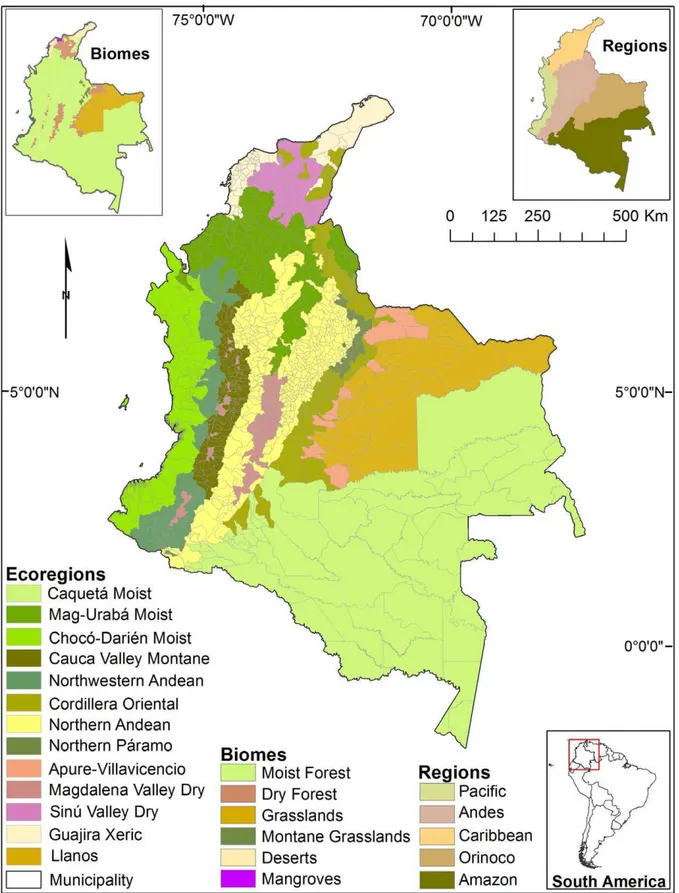
Figure 1. Map of the 13 ecoregions and 1117 municipalities in Colombia.Insert shows the distribution of the six biomes, and the five regions.
sub-national regions. Nevertheless, land cover mapping at the national scale using higher resolution data has major limitations because of difficulties in getting cloud-free images, low temporal resolution, or high cost, and image gaps in the case of Landsat 7 [23]. Some developing countries have produced regional forest monitoring programs (e.g. India and Brazil), including data from their own national satellites with high resolution images from 20 to 70 m (see [21,24]. However, implementing systematic forest assessments such as those in India and Brazil in other developing countries is difficult because of the limitations in technical infrastructure, expertise, and data collection costs [17]. The Moderate Resolution Imaging Spectroradiometer (MODIS) satel-lite data products are reliable and useful tools for monitoring land change in developing countries. Although MODIS has a minimum spatial resolution of 250 m, advantages include: high temporal resolution (i.e., daily) of imagery which can be composited to reduce cloud coverage and rapid data availability at no cost. These characteristics allow a complete LULC mapping not only at the global and national scales, but regional and sub-regional scales as well [18,19,25].
Colombia is one of the most biodiverse countries on Earth [26] especially in the categories of plants, mammals, reptiles, amphib-ians, and birds [27,28]. Colombia also has one of the largest continuous forest areas in the tropics, covering at least 49% of the national land territory [25]. Despite its high biodiversity and natural resources, there is no consistent multi-temporal dataset of LULC change for Colombia. Forest cover assessments are mainly done by two official organizations, the IDEAM (Instituto de Hidrologı´a, Meteorologı´a y Estudios Ambientales) and the IAvH (Instituto de Investigacio´n de Recursos Biolo´gicos Alexander von Humboldt). These organizations provide maps and reports at regional to national scales based on remote sensing products from MODIS and Landsat sensors, but ground-based forest inventories have not been made at the national scale. Another source of information is FAO, which estimates forest cover every five to ten years. The most recent FAO estimates in 2010 are based on 2002 maps provided by IDEAM [29], but FAO adjusts IDEAM data with their own methodology to standardized forest assessment in multiple countries. At regional and local scales, government agencies (e.g. Corporaciones Auto´nomas Regionales), non-gov-ernment organizations (e.g. Fundacio´n Natura), and local and foreign universities also have collected LULC data. Unfortunately, each organization uses their own mapping approaches and different spatio-temporal scales, which makes it difficult to compare LULC data among studies, regions, and years.
Land transformation is not homogeneous in Colombia, but rather varies greatly among its different ecological and political regions [26] (Figure 1). The Andes and the Caribbean regions have been the most impacted as part of the early colonization process (after 1500 AD; [30]) that severely affected its biodiversity and natural resources. However, since 1900 forest clearing has concentrated in the eastern lowlands, mainly in the Amazon and Orinoco regions [31]. Forest cover transformation in Colombia usually begins with the clearing of small areas used for subsistence agriculture, later these areas are often replaced by pastures for livestock grazing; and many of these areas are transformed in to mechanized agriculture (e.g. rice; [32]). Over the years, many such areas have been abandoned due to loss of soil productivity [32,33], rural-urban migration, technology improvement, and globaliza-tion of markets [34]; these processes promote forest recovery, but in some cases these abandoned lands continue in a degraded state [35]. Nevertheless, there is a lack of recent information about how LULC varies across the country and its regions, and between different ecosystems. Thus, there is a need for evaluating land
change at multiple spatio-temporal scales using a consistent methodology across the various ecological and socioeconomic gradients of Colombia.
The purpose of the present study is to assess land change from 2001 to 2010 in Colombia, with a focus on three objectives: (1) determine how land change varies at the country, biome, ecoregion, and municipality scales; (2) identify and analyze the spatial distribution of areas experiencing significant land change; and, (3) discuss the implications of our findings for land use and conservation planning in Colombia. This research was based on a novel method for mapping LULC annually, which coupled MODIS (250 m) products with reference data interpreted from high spatial resolution imagery (QuickBird) in Google Earth that allows us to quantify land change at multiple spatial scales.
Methods
Study Area
Colombia is located in the northwestern part of South America, bordered by the Caribbean Sea to the north and the Pacific Ocean to the west, and occupying an area of 1.1 million km2. Colombia has about 45.4 million people and an average population density of 40.1 people per km2 (see http://www.dane.gov.co). Differences in elevation and latitude produce large climatic variation across the country. For example, there are dramatic differences in annual precipitation, ranging from 350 mm (Guajira peninsula) to 12,000 mm (Pacific lowlands). Consequently, the combination of different climates, elevation ranges, and geographic location have allowed the development of a high diversity of habitats and species richness in Colombia, as well as an array of land uses.
Colombia can be divided into five continental regions (Andean, Caribbean, Pacific, Orinoco, and Amazon; Figure 1), 26 ecoregions, and 63 ecosystems [26]. These regions have remark-able biogeographic, socio-cultural, economic, and demographic differences. Consequently, LULC across the country has under-gone distinct land transitions in the different regions. The Andean region is composed of three mountain ranges (Western, Central, and Eastern) that sustain montane ecosystems with multiple vegetation types. Pasturelands are the dominant land cover in the region (24%) compared with croplands (19%). The Caribbean region is characterized by xerophytic and subxerophytic vegeta-tion types that correspond to arid and semiarid lowland areas. Lands in the Caribbean are mainly used for cattle ranching (48%) and another considerable fraction for agriculture (14%). The Pacific region contains a dense coastal lowland rain forest, where croplands cover a greatest area (10%) compared with pasturelands which cover less than 2%. In the Orinoco region (usually referred to as the Llanos), pasturelands (86%) and croplands (3%) have increased rapidly since the 1980’s. Finally, the Amazon, the largest and least transformed region of the country, is mostly covered by tropical rainforests; however, previous studies have estimated that deforestation has converted about 6% of forests into pasturelands, and less than 1% into legal and illegal croplands [36].
In this study, municipalities (second administrative level) were the main unit of analysis. According to the National Administra-tive Department of Statistics (DANE) data, the number of municipalities in Colombia was 1,100 in 2007. However, we included 1,097 municipalities instead of 1,100 because three municipalities were created after the last census in 2005. We also included 20 areas no municipalizadas orcorregimientos (name of the third administrative level in Colombia) because they occupied a large area (almost 190,000 km2) in the southern portion of the
analyses were thus performed on 1,117 municipalities or study units.
Land-use/land-cover Mapping
Our LULC classification methodology generally follows those first outlined by [18] and modified for continental-scale mapping in [37]. Here we summarize the three main steps that pertain to the Colombian national maps used in our analysis:
(1) Google Earth reference data collection (.10,000 samples): reference data for classifier training and accuracy assessment were collected with human interpretation of high-resolution imagery in Google Earth (GE, http://earth.google.com) mainly from Digital Globe’s QuickBird satellite (http:// www.digitalglobe.com) spanning 2001 to 2010 [38]. Visual interpretation methods followed those in [18,38] and were performed by the authors (AMSC, M.A, and M.C) and student technicians. Samples were 2506250-m areas placed manually across the tropical and subtropical moist broadleaf forests, tropical and subtropical dry broadleaf forests, and tropical and subtropical grasslands, savannas and shrublands biomes [39], which covered Colombia and extended into neighboring countries [38] (Figure S1). Samples were located with both random sampling and stratified random sampling, which included areas with mixed cover types, and samples well within patches of homogeneous cover, and no two samples were closer than 1,000 m apart [38]. Prior to interpretation, sample centers were snapped to the closest satellite image pixel (MODIS). Each sample class was assigned the year of the image and the percent cover of seven cover classes was visually interpreted: woody (woody vegetation including trees and shrubs); herb (herbaceous vegetation); ag
(agriculture);plant(plantations);built(built-up areas);bare(bare areas); and water. If two interpreters agreed on the majority cover and GE image year of a sample, then their percent cover estimates were averaged. If the interpreters disagreed on the majority cover or year (mostly cover), then an ‘‘expert’’ (author) estimated the final class cover and recorded the year [38]. Samples were assigned to a class if the cover in this class was$80%. Samples with 20–80%woody, with abare,herborag
component,80% were assigned to amixed woodyclass. (2) Satellite imagery used in classification: we used the MODIS
MOD13Q1 Vegetation Indices 250 m product (Collection 5) for LULC classification [18,37]. The product is a 16-day composite of the highest-quality pixels from daily images and includes the Enhanced Vegetation Index (EVI), red, near infrared (NIR), and mid-infrared (MIR) reflectance and pixel reliability [40]. Twenty-three samples were available per year, with data available from 2001 to present. All MODIS scenes were reprojected from their native Sinusoidal projection to the Interrupted Goode Homolosine projection (sphere radius of 6,378,137.0 m) using nearest-neighbor resampling. The original cell size of 231.7 meters was maintained in the reprojection. For each pixel, we calculated the mean, standard deviation, minimum, maximum, and range statistics for EVI, and red, NIR and MIR reflectance values for calendar years 2001 to 2010. Statistics were calculated for all 12 months, 2 six-month periods, and 3 four-month periods. The MOD13Q1 pixel reliability layer was used to remove all unreliable samples (value = 3) prior to calculating statistics. If fewer than three samples were available for a statistics temporal window for a given year, then the statistics for that window were given null values.
(3) Mapping LULC with the Random Forest classifier: we mapped LULC with the Random Forests (RF) tree-based classifier [41] following methods in [37]. An advantage of the RF classifier is that it provides an assessment of error with ‘‘out-of-bag’’ (OOB) samples, a form of multi-fold cross-validation [18,41]. These data can be used to calculate an error matrix, an unbiased estimate of accuracy, rather than withholding samples in an independent test dataset [18,41]. RF classifier was implemented using R (v. 2.12.2; [42]) and therandomForestpackage (v. 4.622; [43]) with 1999 decision trees, a minimum of 5 samples in terminal nodes (node-size = 5), and sqrt(p) as number of variables randomly sampled as candidates at each split, wherep is number of variables (mtry = default). Predictor variables were MODIS-based 4-, 6-and 12-month statistics for EVI, red, NIR 6-and MIR, 6-and were extracted for the year corresponding to the QuickBird image year (range 2001 to 2010 [38]) for each GE reference sample. We trained four separate RF based on samples in separate biomes with boundaries defined by municipalities. The tropical and subtropical moist broadleaf forests biome was split to include an Amazon basin section and a coastal lowlands section, while the desert and xeric shrublands biome was combined with the tropical and subtropical dry broadleaf forest biome [37,38] (Figure S1). An initial RF for a biome was generated with the reference data class and MODIS predictor variables from that biome. Theoutlier function in randomForest was used to eliminate samples with an outlier metric greater than 10, and a final RF was generated from the remaining samples, leaving 10,143 of 10,622 (96%) samples for training the final RF (Table 1). We used R and the RGDAL library to apply the RF objects to every pixel in MODIS tiles covering the zone-biome region for each year, 2001 to 2010. For a given year, if a pixel had valid 4-, 6- and 12-month statistics, then the class was assigned based on the initial RF; a secondary RF based on just 12-month statistics was applied to pixels that had only valid 12-month statistics; and, the pixel was assigned a No Data value if it had no valid predictor variables (e.g., areas with persistent cloud cover, beach/water interfaces along coasts). On average each annual map had 0.14%60.09% of the area covering Colombia mapped as No Data. Pixels with $4 No Data values over 10 years were set to a null value and excluded from our maps, as these were unreliable areas for mapping – mostly coastal areas in Colombia. The four separate maps were then mosaicked and reclassified (post-classification) by groupingag
and herb, mixed woody and plant, and built and bare. The combining of classes into a five-class scheme helped reduce inter-class confusion and increase map accuracy while still allowing us to focus on major trajectories of change inwoody
vegetation. Based on the OOB statistics, the final five-class maps had an average overall accuracy of 87.4% (64.3%), with non-water average producer’s accuracies ranging from 36.3% (mixed woody/plant) to 96.9% (woody) and user’s accuracies ranging from 72.5% (mixed woody/plant) to 89.4% (woody) (Table 2). The five-class LULC map was then summarized for the 1,117 municipalities.
Land Change Dynamics
2010). If more than 1% of the total municipality area had pixels mapped as No Data for a given year, then the land cover data for that year were removed from the regression. To determine the strength of this linear relationship we used Pearson’s correlation coefficient (R), where positive values of R represent an increase in a LULC cover and negative values of R represent a decrease. We used this approach to standardize land change through time due to outliers or missing data in any given year, and the use of R for trends allows us to compare municipalities, which can vary in size from 17,6 km2to 65,568 km2. In addition, this trend analysis takes advantage of the ten years of data, and it is not based on just two points in time. Municipalities with significant changes in any cover had p#0.05. All analyses incorporating absolute area were performed using estimates based on the each municipality’s regression model, rather than the raw area data used to fit the model.
We calculated the net change in cover (km2) of the three classes between 2001 and 2010 considering four scales: country, biome, ecoregion, and municipality. Biome and ecoregion scales were established following the World Wildlife Fund biome and ecoregion framework [39]. We clustered municipalities into the six major biomes and 25 ecoregions that were described for Colombia (Table S1). Municipalities present in more than one biome and ecoregion were classified as the unit with the greatest area in each municipality. We included tropical and subtropical moist broadleaf forest (Moist Forest), tropical and subtropical dry broadleaf forest (Dry Forest), tropical and subtropical
grassland, savanna and shrubland (Grassland), Montane Grass-land and ShrubGrass-land (Montane GrassGrass-land), Desert and Xeric Shrubland (Desert), and Mangrove (Mangrove) biomes. We reduced the 25 ecoregions to 13 because some ecoregions were represented by only one or a few municipalities (Figure 1). For example, Western Ecuador Moist Forest (NT0178) was present in only one municipality (Tumaco). Therefore, this municipality was aggregated to the largest and closest ecoregion (Choco´-Darie´n Moist Forest/NT0115), which also contained similar environmental characteristics. We performed a Mann-Whitney test in R (v. 2.12.2; [42]) to determine if there was a significant difference in the size of municipalities that gained or lost woody
vegetation.
Results
Land-use/land-cover Change from 2001 to 2010
At the country level,woodyvegetation was the most predominant land cover (Figure 2).Woodycover increased from 580,420 km2in 2001 to 597,383 km2in 2010, with a net gain of 16,963 km2.Ag/ herbclass also increased from 383,097 km2to 397,741 km2with a net gain of 14,644 km2. In contrast,mixed woody/plant decreased from 151,930 km2in 2001 to 122,648 km2in 2010, with a net loss of 29,282 km2.
At the biome level,woodycover only decreased in the Grasslands biome (1,636 km2), while it increased in the other five biomes, from 16,077 km2in the Moist Forest, to 57 km2in the Montane
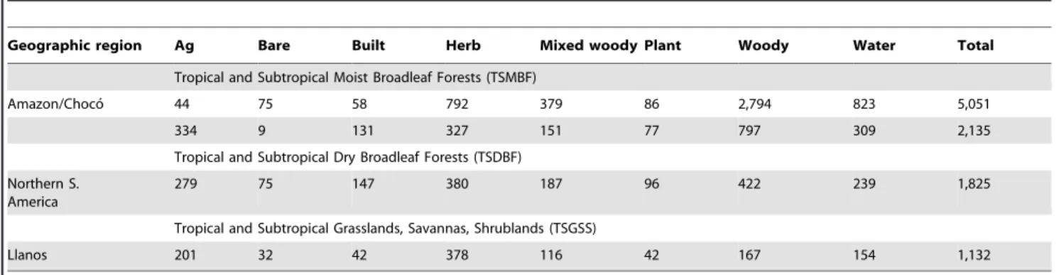
Table 1.Mapping regions and total sample counts used in each separate Random Forest (n = 4).
Geographic region Ag Bare Built Herb Mixed woody Plant Woody Water Total
Tropical and Subtropical Moist Broadleaf Forests (TSMBF)
Amazon/Choco´ 44 75 58 792 379 86 2,794 823 5,051
334 9 131 327 151 77 797 309 2,135
Tropical and Subtropical Dry Broadleaf Forests (TSDBF)
Northern S. America
279 75 147 380 187 96 422 239 1,825
Tropical and Subtropical Grasslands, Savannas, Shrublands (TSGSS)
Llanos 201 32 42 378 116 42 167 154 1,132
These include only samples filtered by the Random Forest outlier removal step (Biomes follow Olson et al. 2001). doi:10.1371/journal.pone.0043943.t001
Table 2.Classification accuracy assessment.
Producer’s Accuracy (%) User’s Accuracy (%)
Biomes Samples
Overall
(%) Ag/Herb Bare/Built
Mixed woody/
plant Woody Water Ag/Herb Bare/Built
Mixed woody/
plant Woody Water
Moist Forest1 5,051 92.2 86.5 64.7 49.7 100.0 99.9 78.7 86.9 73.6 97.7 95.8
Moist Forest2 2,135 89.2 90.5 91.4 33.3 99.6 100.0 83.5 89.5 71.0 92.6 99.0
Dry Forest3 1,825 82.0 87.3 90.1 32.5 92.4 100.0 78.6 82.6 68.7 81.6 100.0
Grasslands4 1,132 86.1 97.4 67.6 29.7 95.8 100.0 83.9 89.3 77.0 86.0 98.1
Total/Avg 10,143 87.4 90.4 78.4 36.3 96.9 99.9 81.1 87.0 72.5 89.4 98.2
Biome description:
1Tropical and Subtropical Moist Broadleaf Forest (Amazon basin section). 2Tropical and Subtropical Moist Broadleaf Forest (Coastal lowlands section). 3Tropical and Subtropical Dry Broadleaf Forest.
Grasslands (Figure 2). Themixed woody/plantclass in turn, increased only in the Desert biome (621 km2), while there was a large decrease in the Moist Forest biome (27,181 km2). The ag/herb
cover only decreased slightly in Mangroves (21 km2), while increasing in the rest of biomes from 10,652 km2 in the Moist Forest to 58 km2in the Dry Forest.
In 2001 and 2010,woodyvegetation was the dominant cover in four ecoregions, whileag/herbvegetation was the dominant cover in nine ecoregions (Figure 2). Land cover change varied greatly
among ecoregions. Woody vegetation decreased only in Apure-Villavicencio and Llanos ecoregions with a reduction of 691 km2 and 1,636 km2, respectively. In the other eleven ecoregionswoody
vegetation increased, seven of which had a net gain of more than 1,200 km2. The net gain varied from 4,535 km2in the Northern Andean forests to 63 km2 in the Northern Pa´ramo ecoregions. The Caqueta´ Moist forest ecoregion, the largest ecoregion in Colombia (472,066 km2) also had a small increase in woody cover (144 km2) when compared with the rest of the ecoregions.Mixed
Figure 2. Absolute area ofwoodyvegetation (W),mixed woody/plant(MWP), andag/herb(AH) from 2001 to 2010 at the country, biome (B) and ecoregion (E) scales. These estimates are based on estimates from municipality-scale regression models and include all municipalities.
woody/plant class increased only in the Guajira Xeric ecoregion (552 km2), and decreased in more than 1,500 km2 in eight ecoregions.Mixed woody/plantnet loss varied between 7,147 km2in the Magdalena-Uraba´ Moist forest and 9 km2in the Magdalena Valley Dry forest ecoregions. The ag/herb vegetation mainly decreased in the Sinu´-Valley Dry forest (1,347 km2), the North-western Andean (969 km2), and the Cauca-Valley Montane forest (310 km2). The net gain in ag/herb vegetation varied between 5,256 km2 in the Caqueta´ Moist forest and 25 km2 in the Magdalena-Valley Dry forest.
At the municipality level,woody vegetation increased in 73% (820) of the municipalities with a net gain of 28,092 km2, and decreased in 24% (264) of the municipalities with a net loss of 11,129 km2 (Table S2). In contrast, the mixed woody/plant class increased in 31% (347) of the municipalities with a net gain of 5,199 km2, while it decreased in 68% (762) of municipalities with a net loss of 34,481 km2. For the ag/herb class, the number of municipalities gaining (53%; 587) and losing (47%; 526) cover was similar, but the area gained was almost double (28,345 km2) of that lost (13,701 km2). We also found that 21% (232) of the municipalities showed significant change in woody vegetation during the last decade. This percentage was similar for mixed woody/plant (23%; 254) and for ag/herb (20%; 225). If we only considered municipalities with significant changes during the last decade, we detected a close correspondence between loss and gain ofwoodyvegetation,mixed woody/plant,andag/herbclasses (Figure 3). Examples of this dynamic include: i) areas wherewoodyvegetation was transformed into ag/herb in the southern part of the Magdalena Medio and the Llanos piedmont regions; ii) transitions fromag/herbvegetation towoodyvegetation were located in western Cundiboyacense highplain, and between Nudo de los Pastos and the Macizo Colombiano (Figure 3A); iii) transitions from mixed woody/plant to ag/herb vegetation appeared in the Magdalena Medio and the Alto Caqueta´ regions; iv) transitions fromag/herb
vegetation to mixed woody/plantwere located only in the north of the Cundiboyacense highplain (Figure 3B); v) transitions from
woody tomixed woody/plant was not common; and, vi) transitions from mixed woody/planttowoody vegetation were concentrated in the Catatumbo and to the north of the Magdalena Medio, as well as to the north of the central and western Andean mountain ranges (Figure 3C). The average size of the municipalities that significantly gained or lost woody vegetation was 688 km2 and 3,113 km2, respectively, and this difference was significant (Mann-Whitney U = 3.6,p= 0.0003).
Finally, to determine the hotspots ofwoodyvegetation change we selected the top 10 municipalities with the greatest net gain or loss in woody cover (Table 3). The top 10 municipalities with the greatestwoodyvegetation gain account for 14% of the totalwoody
increase, and 42% of the increase when only considering municipalities with a significant change in woody vegetation. Interestingly, Cumaribo, the largest municipality in Colombia, accounted for almost 4% of total increase inwoodyvegetation and 11% considering municipalities with a significant gain. The 10 municipalities with the greatestwoodyvegetation loss account for 27% of total decrease, and 91% of municipalities with a significant loss inwoodycover. Municipalities showing the greatest net gain were located primarily in the Magdalena-Uraba´ Moist forest and Choco´-Darie´n Moist forest, while those with the greatest net loss were located mainly in the Llanos, Apure-Villavicencio, and Northern Andes.
Discussion
Patterns of Land Cover Change at the Country Level
Our results show that during the last decade, land change in Colombia has been characterized by an unexpected net gain in
woodycover, increasing by 16,963 km2or 3% of its initial area in 2001. In contrast, previous literature has highlighted dramatic forest loss at the national [22] and regional scales [32,44].Woody
cover as well asag/herbclasses expanded mostly at the expense of themixed woody/plantclass at the national and municipality levels. At first glance, it appears that woody regrowth results from secondary forest/shrub recovery rather than recently abandoned agricultural areas. Forest regrowth at the national scale is consistent with the general reforestation trends in Europe, the U.S.A. [45], and in other Latin American countries such as Ecuador, the Dominican Republic, Puerto Rico, Costa Rica [11– 14]. However, secondary vegetation regrowth in Colombia might be the effect of land abandonment resulting from armed conflicts and economic development experienced during the last 10– 20 years [46]. Land abandonment of rural areas began in the early 1990s when the Colombian government implemented an economic liberalization model, and it continued in the late 1990s as a result of the intensification of internal conflicts. The effects of these conflicts and the associated political decisions have been documented for the Caqueta´ region [47]. Although the amount ofwoodyvegetation gained was almost three times higher than the amount of forest lost, it is clear that deforestation continues. Extensivewoodycover losses occurred in municipalities principally to the southwest of Magdalena Medio (e.g. Segovia and Remedios) and in the Llanos regions (e.g. San Luis de Palenque, Tame), where 3,000 km2of woody vegetation were converted to croplands and pastures. Deforestation in these areas is related to gold mining and oil exploitation activities, and agricultural expansion. For example, in the Magdalena Medio region woody
vegetation has been cleared for small-scale agriculture and timber extraction by miners since the 1990s [48]. In the Llanos, the construction of the Villanueva-Yopal road and the road infrastructure to aid oil exploration has stimulated the expansion of trading, cattle, and agriculture. For example, rice cultivation has increased from 1,300 km2in 2001 to 1,800 km2in 2009 [49]. The decrease inwoodyvegetation in these regions affects areas of global importance for biodiversity such as Serranı´a de San Lucas located to the south of Magdalena Medio [48] and along the Andean foothills in the Llanos.
also includes shrubs, palms, and bamboo, but not tree plantation [22]. In contrast, our definition of forest or ‘‘woody’’ vegetation differs from the former definitions because we include trees and shrubs, (i.e., no height requirement) with $80% cover. Consequently, our definition of mixed woody
vegetation (20–80% woody) combined with plantations is more comparable to FAO’s and IDEAM’s definition of ‘‘forest’’. In addition, FAO and IDEAM estimates showed the same deforestation trend because their definitions of forest are somewhat similar and FAO results are typically based on existing maps provided by IDEAM [29]. Nevertheless, IDEAM maps in 2000, 2005, and 2010 lacked information for approximately 8% of Colombia due to cloud coverage. Thus,
conclusions drawn from these maps could be misleading in either direction with regard to forest cover. These areas without information from IDEAM were scattered across the country, particularly in the north portion of the Pacific region and areas spread throughout the Andes and the Amazon regions where cloud cover is high, and where at the same time we found the largest net gain inwoody vegetation.
In general, our methodology to map annual LULC in Colombia, which combined MODIS products, Google Earth reference data, and Random Forest classifier [37], provides a consistent classification scheme at multiple spatial-temporal scales. The high accuracy values we obtained demonstrate the robustness of the mapping method and the reliability of our LULC maps
Figure 3. Areas of significant change in land cover.Transitions between A)woodyvegetation and ag/herb; B)mixed woody/plantandag/herb; C)woodyvegetation andmixed woody/plantare shown. Red and blue dots represent municipalities with significant loss and gain in cover area (km2), respectively. Black ovals represent prominent clusters of land cover change. Orange and green arrows present deforestation and reforestation transitions, respectively. Land transitions (i–vi) discussed in the text.
which have several advantages with respect to previous maps, including: (1) quantification of both deforestation and reforestation patterns across the country at multiple spatial scales; (2) using Google Earth reference data collection for classifier training and accuracy assessment (rather than ground-based reference data collection) which provides us a fast and inexpensive way to acquire reference data across the whole country, a large part of which is difficult to access; (3) use of temporally-composited MODIS data, which greatly reduces the amount of pixels adversely affected by
cloud coverage and thus allows wall-to-wall LULC change monitoring; and, (4) leveraging 10 years of annual LULC area at municipality level to better estimate 2001 to 2010 net change, thus reducing the influence of climate fluctuations or other factors that could bias analyses based on just two years of data, and to determine which municipalities had significant increases or decreases in area while normalizing differences in municipality area.
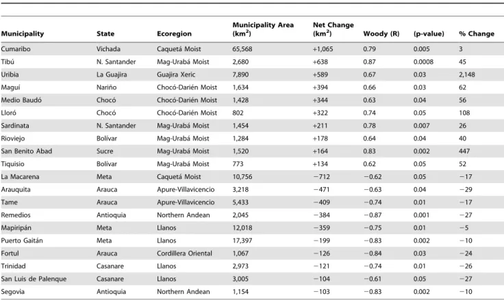
Table 3.Top ten municipalities with the greatest net gain (+) and net loss (2) ofwoodyvegetation between 2001 and 2010.
Municipality State Ecoregion
Municipality Area (km2)
Net Change
(km2) Woody (R) (p-value) % Change
Cumaribo Vichada Caqueta´ Moist 65,568 +1,065 0.79 0.005 3
Tibu´ N. Santander Mag-Uraba´ Moist 2,680 +638 0.87 0.0008 45
Uribia La Guajira Guajira Xeric 7,890 +589 0.67 0.03 2,148
Maguı´ Narin˜o Choco´-Darie´n Moist 1,634 +394 0.66 0.03 62
Medio Baudo´ Choco´ Choco´-Darie´n Moist 1,428 +344 0.63 0.04 56
Lloro´ Choco´ Choco´-Darie´n Moist 802 +322 0.74 0.05 108
Sardinata N. Santander Mag-Uraba´ Moist 1,454 +211 0.78 0.007 26
Rioviejo Bolı´var Mag-Uraba´ Moist 1,284 +178 0.64 0.04 40
San Benito Abad Sucre Mag-Uraba´ Moist 1,520 +164 0.83 0.002 447
Tiquisio Bolı´var Mag-Uraba´ Moist 773 +134 0.62 0.05 52
La Macarena Meta Caqueta´ Moist 10,756 2712 20.62 0.05 217
Arauquita Arauca Apure-Villavicencio 3,218 2471 20.63 0.04 229
Tame Arauca Apure-Villavicencio 5,433 2409 20.74 0.01 217
Remedios Antioquia Northern Andean 2,045 2384 20.87 0.001 227
Mapiripa´n Meta Llanos 12,018 2359 20.75 0.01 25
Puerto Gaita´n Meta Llanos 17,397 2199 20.83 0.002 210
Fortul Arauca Cordillera Oriental 1,067 2126 20.84 0.03 224
Trinidad Casanare Llanos 2,973 2121 20.74 0.01 226
San Luis de Palenque Casanare Llanos 3,005 2104 20.61 0.05 227
Segovia Antioquia Northern Andean 1,154 2103 20.83 0.002 210
Columns show area, net change, correlation coefficient (R),p-value, and the percentage of change of the top ten municipalities with greatest net gain and loss between 2001 and 2010.
doi:10.1371/journal.pone.0043943.t003
Table 4.A comparison of four estimates ofwoodyvegetation class at the national scale.
Woody vegetation area (km2)
Year This study (W){
This study (W+MWP){
IDEAM1 FAO2 MOD44B3(VCF 500 m){
MOD44B3(VCF 500 m)±
2000 n.a. n.a 617,328 615,090 269,195 820,392
2001 580,420 732,350 n.a. n.a. 298,170 839,487
2005 587,953 726,817 602,063 610,040 352,710 832,261
2008 593,611 722,723 n.a. n.a. n.a. n.a.
2010 597,383 720,031 586,336 604,990 n.a. n.a.
{
Data including onlywoodyvegetation. {Data including
woodyvegetation+mixed woody/plant.
{
Forest cover (80 crown cover).
6Forest cover (25 crown cover).
Sources:
1Cabrera E, Vargas DM, Galindo G, Garcı´a MC, Ordon˜ez MF, et al. (2011). 2FAO (2010) Global Forest Resources Assessment 2010.
We acknowledge that there are two potential caveats to our study. First, MODIS pixels will not detect small-scale changes (e.g. slash and burn agriculture,,5 ha) due its lower spatial resolution. However, the accumulative change from the small-scale conver-sion can be captured by our 10-year trend analysis based on the aggregation of all pixels within a municipality. Although Landsat provides higher spatial resolution which facilitates detection of small-changes, there are major gaps due to clouds cover that make it difficult to map the whole country using Landsat imagery. Second, using reference data from QuickBird imagery in Google Earth could include interpretation and spatial error. For example, visual interpretation of some land cover classes in Google Earth is difficult, and therefore, our cover classes were very general. Even though our classes were relatively easy to identify, interpreters sometimes disagreed onag andherbsamples for which an expert determined the final class label. Additionally, spatial error can be the result of terrain distortions especially in QuickBird images that have not been orthorectified. However, it has been shown that QuickBird scenes are very accurate with an average error of 10 m of disagreement between ground control points and GE QuickBird images [18].
Potential Factors Explaining Woody Vegetation Recovery
There are three potential factors that could explain the increase inwoodyvegetation observed in our LULC maps. The first possible explanation could be an increase in oil palm plantations. Oil palm plantations have expanded rapidly since the 1990s when Colombia initiated its economic liberalization model [51]. According to the The National Federation of Oil Palm Growers (Fedepalma), palm plantations for oil extraction increased from 180 km2in the 1960s to almost 3,600 km2in 2010– mainly in the Meta, Casanare, Cesar, Magdalena, Bolı´var, Cundinamarca, Santander, Norte de Santander, and Narin˜o departments. Nevertheless, we do not believe that oil palm plantations are an important component of thewoodyrecovery we described. First, we classified plantations separate from woody vegetation. Second, municipalities identified by IGAC [52] as having large areas of oil palm plantations do not coincide with the municipalities we identified as important areas of reforestation. In fact, our results showed that from 2006 to 2008, 76% of the municipalities had net gain inwoodyvegetation (total of 4,740 km2). However, during the same period of time, only 7% of the municipalities had a net gain in palm oil plantations (362 km2; [52]). In addition, taking into account the ten municipalities with the greatest net gain inwoody
vegetation from 2006 to 2008, only Tibu´ (net gain of 142 km2) and Riohacha (net gain of 81 km2) have oil palm plantations (net gain
of 50 and 3 km2, respectively; [52]).
A second factor that could explainwoodyrecovery is coca crops eradication programs. At the national scale, coca cultivation area dropped from 1,448 km2 in 2001 to 618 km2 in 2010 [53]. Eradication programs, both manually and by aerial spraying, have been implemented intensively in several localized areas of lowland forests in the Moist Forest biome. Eight of the top 10 municipalities with the greatest net gain in woody vegetation cultivated coca in 2001 (189 km2; [53]). By 2010, the area of coca in these municipalities declined to 58 km2. The majority of this decline occurred in Cumaribo and Tibu´ municipalities, which lost 128 km2of coca plantations between 2001 and 2010. It is possible that we are detecting the first stages of natural regeneration (i.e. shrubs) following the eradication of these illicit crops.
The third potential factor that could explain the increase in
woody cover, particularly in seasonal forests (i.e. dry forests), is related to the inter-annual variation in precipitation. In these areas, anomalous rainfall years (e.g. La Nin˜a events) could change
the vegetation greenness trends detected by MODIS sensors. This phenomenon could changewoody vegetation to mixed woody and vice versa, especially for pixels near the 80% decision threshold. However, we attempted to minimize this effect using regression models by municipality, capturing 10-years of real trends in vegetation dynamics. It would be desirable to use high resolution data such as Landsat to evaluate the accuracy in our LULC maps and to verify observed land change; however, on an annual basis it is difficult to obtain the necessary temporal data for the entire country for detecting any climatic anomalies.
In summary, the national assessment of land cover change in Colombia indicates that woody vegetation gains occur in small municipalities and exceed woody vegetation losses occurring in large municipalities. This scale of analysis gives a valuable general overview of current land change, but it can maskwoodyvegetation losses in some areas. National scale analysis does not take into account intrinsic differences (e.g. socioeconomic, demographic, and biophysical) among regions which can promote different land cover patterns and dynamics. Therefore, by examining data at the biome and ecoregion scales it is possible to decipher where and to what extent changes in woody vegetation are occurring, and to better understand the underlying environmental and social drivers of this change.
Patterns of Land Cover Change at the Biome and Ecoregion Scales
Moist forest biome. This biome accounts for 86% of the total increase inwoodycover. It is the largest biome in Colombia (Table S1) consisting of seven ecoregions which contain both montane forest (4 ecoregions) and tropical forest (3 ecoregions). This recovery occurred mostly frommixed woody/plant, generated in previous periods and less directly fromag/herbvegetation (Figure 2). The net gain in woody vegetation was located especially in the montane forest of the Andes mountain ranges (70%) and in the tropical forest in the Amazon and the Pacific regions (30%). Other studies have quantified forest regrowth in Colombia from secondary vegetation and abandoned pastures, particularly in the Amazon [54] and in the Andes regions [22]. This pattern of forest regrowth in the Moist Forest Biome has also been reported for Venezuela and Costa Rica [55] but, deforestation continues to be the major trend in this biome. These contrasting dynamics are driven by multiple factors including an increase in the global demand for meat (deforestation), as well as the abandonment of marginal agriculture lands and changing patterns of precipitation [55–57].
The four montane forest ecoregions (in the Moist Forest biome) located in the Andes mountain ranges contributed 65% of the total net gain in woody vegetation in Colombia, particularly in the Northern Andean (27%), the Northwestern Andean (22%), and Cauca-Valley (11%) Montane Forest ecoregions.Woodyvegetation increases are likely explained by human causes such as the abandonment of traditional productive systems in the 1990s due to harsh environmental conditions (e.g. arid areas) and globalization processes which have promoted strong rural migration in many municipalities [58]. For example, 43% of municipalities located in the Chicamocha region (Northern Andean ecoregion) lost population between 1993 and 2005 (see http://www.dane.gov. co), and the area is now experiencing significant change frommixed woody/plant class to woody vegetation (mostly shrubland cover; Figure 3C). Similar abandonment patterns can be observed in the Cundiboyacense highplains (Northern Andean ecoregion) where many municipalities are transitioning primarily from ag/herb to
explain part of thewoodyincrease in this area. These factors have also facilitated a significant reforestation (transitioned fromag/herb) of large expanses of montane forest to the south of the Northwestern Andean (between the Macizo Colombiano and Nudo de los Pastos) and to the north of the Cauca-Valley Montane forest ecoregions as well. This reforestation trend has been seen in both developed and developing countries, supporting the idea that the abandonment of less productive lands and the globalization of markets may lead to the regrowth of secondary forest [61,62].
All three ecoregions in the Moist Forest biome experienced gains inwoodyandag/herbvegetation, which transitioned from the
mixed woody/plant vegetation class. For instance, the Magdalena-Uraba´ Moist Forest ecoregion showed a remarkable decrease in
mixed woody/plant class, particularly in the Magdalena Medio region where 46% transitioned to woody vegetation and 44% transitioned toag/herbvegetation, the remaining area transitioned to other classes (i.e.built-upandbare soil).Woodyvegetation in the Caqueta´ Moist forest ecoregion seems to be stable, contributing only 0.8% of the total net gain inwoodyvegetation in Colombia. These results coincide with data from the Amazon forest, which showed forest regrowth transitioned primarily from previous croplands [44]. However, our findings contrast with the IDEAM results that include the Amazon region as one of the deforestation hotspots of the country [22]. But, if we combine our woody
vegetation andmixed woody/plantclasses, which is more comparable with the definition of forest used by IDEAM, we detect a loss of .5,000 km2. Virtually all of this change is frommixed woody/plant
toag/herb. These losses in the Caqueta´ Moist forest are the result of small-scale subsistence agriculture (driven by rural-rural migration [63] and illicit crops, particularly in the Alto Caqueta´ in the Caqueta´ department.
Grasslands biome. This is the second largest biome in Colombia and includes only the Llanos ecoregion. The Llanos is increasingly being considered as the new agricultural frontier of Colombia (see: http://webapp.ciat.cgiar.org/es/descargar/pdf/ convenio_colombia_ciat.pdf). Large woody vegetation losses were located mainly in the central area of Casanare and the eastern area of Meta departments where an intense land conversion is associated with human population change and investments in infrastructure to support an important oil exploration activity and agricultural intensification. High rates of land conversion (towards mechanized agriculture and cattle grazing) corresponding with urban population growth and migration have been registered since the 1980s [64], a pattern that appears to continue today. Between 1993 and 2005, 92% of the municipalities gained people (see http://www.dane.gov.co) and 85% gained ag/herb vegetation, implying that agriculture (e.g. rice) and pastures are still expanding, as in many other regions [65,66]. Nevertheless, the transformation of savannas in the Orinoco region, which is steadily increasing and currently a major land use change in Colombia [67], cannot be quantified with our method as it will be a transition from herbaceous vegetation to agriculture, which are both contain in our combined ag/herb class. Changes are only detected when the change is to perennial plantations.
Dry forest biome. This is the third largest biome and includes three ecoregions: Magdalena Valley, Sinu´ Valley, and Apure-Villavicencio Dry forest. This biome accounts for 4% of the total increase inwoodyvegetation and its recovery was the result of a transition mostly fromag/herbvegetation in the Sinu´ Valley Dry forest. From 1990 to 2003, the cotton industry decreased in the Sinu´ valley due to changes in pricing policies and competition with the subsidized international markets that significantly affected its area and production. Consequently, this crop had an annual loss rate of 13% of cultivated land between 1990 and 2003 [68]. The
Apure-Villavicencio Dry forest ecoregion showed a decrease in
woodyvegetation as a result of agriculture and pastures expansion (as in the Llanos ecoregion). This expansion was located particularly in the foothills of the Arauca department where the majority of the population is located. According to the DANE censuses, 93% of the municipalities in the Apure-Villavicencio Dry Forest ecoregion gained people between 1993 and 2005 and 87% gained ag/herb vegetation. We believe that the expansion of intensive agriculture and cattle pasture will continue as a major driver of deforestation in this region.
Desert and mangroves biomes. These biomes only include the Guajira Xeric ecoregion which had a net gain in woody
vegetation. These biomes account for 9% and 0.7% of the national increase inwoody vegetation, respectively. The increase in woody
vegetation in the Desert biome was concentrated in three municipalities that alone account for 73% of the total increase in this biome. The gain inwoodyin these municipalities could be related to a precipitation anomaly (e.g. 2009) or perhaps a problem in the classification given that the Desert biome was classified as part of the Dry Forest biome (Table 2). Woody
regrowth (mostly shrubland cover) in the Deserts have been reported in Mexico and U.S as a result of the increase in annual precipitation and the decrease of fire and grazing, respectively [57,69]. On the other hand, in the Mangrove biome,woodygains are likely the result of the implementation of conservation and management strategies of mangrove ecosystems across the country [70]. For example, the increase inwoodyvegetation was located in two municipalities (98% of the total increase in this biome) that contain the Vı´a Parque Isla de Salamanca protected area, which was declared a Ramsar Site in 1998 and Reserve for Humankind and the Biosphere by UNESCO in 2000 (see http://www. parquesnacionales.gov.co).
Montane grasslands biome. This biome includes the Northern Andean Pa´ramo ecoregion which had a slight increase in woody vegetation, accounting for only 0.3% of the national increase in woody vegetation. The gain could be the result of regrowth in areas previously occupied byPapaver somniferum(poppy) plantations. Between 1993 and 2008, the area in poppy fields decreased from 75 km2 to 4 km2 across Colombia [71]. This biome has also experienced a significant increase in ag/herb
vegetation. The gains in ag/herb cover were located mainly in municipalities in the Santander and Boyaca´ departments where potato farming and cattle grazing are important activities. In these departments, the cultivated area of potatoes increased from 380 km2to 482 km2between 2006 and 2008 [52] in response to the national and international demand for potato products. Since the potato is the agricultural product with highest consumption per capita in Colombia [72], its cultivation is expected to expand in the near future, adding more pressure on the Pa´ramo ecosystems.
Implications for Conservation Planning
highest rates of woody vegetation loss. These areas have had extensive areas of natural savanna vegetation transformed to crops and pastures during the past 20 years [64,67]. We suggest that a primary conservation goal in Colombia should be the implemen-tation of protected areas in these regions. The Llanos ecoregion is particularly important given its heterogeneous landscapes, its high diversity of vegetation types, and its large numbers of plants, amphibians, reptiles, and fish [75]. Not surprisingly, this ecoregion has been cataloged within the Global 200, which is a set of the most outstanding ecoregions for global conservation [75]. In addition, the Apure-Villavicencio dry forest should be taken into account in the protected areas network because it represents the transition zone between the Andean foothills and the llanos savannas where a relatively high number of plant, reptile, and bird species (including several endemics) coexist (See http://www. worldwildlife.org/wildworld/profiles/terrestrial_nt.html# trop-grass). We also documented a large decrease inmixed woody/plant
in the Magdalena-Uraba´ Moist forest ecoregion, particularly in the Magdalena Medio region. The increase in agriculture and pastures combined with ongoing illegal logging activities [70,76] have endangered a great number of native timber species (e.g.
Libidibia ebano, Cariniana pyriformis). This region should be considered for the protected area network given that there is only one reserve (Serranı´a de los Yariguı´es national park) in this region. On the other hand, the recovery of woody vegetation in the Andes Mountain Ranges is an excellent opportunity to comple-ment, expand and interconnect the protected areas to create a conservation network across the rural landscape mosaics in the region. A relevant area for conservation is the Northern Andean Montane Forest ecoregion, which is also included in the Global 200 [75]. In this ecoregion, the Cundiboyacense highplain had a substantial and significant gain ofwoodyvegetation between 2001 and 2010. Other authors have stressed the importance of this region as a priority area for conservation due to its large areas of land transformation and large number of species at risk [74]. We also highlight that even though the Northern Andean Pa´ramo ecoregion gained slight amounts ofwoodyvegetation, the gains in theag/herbclass were almost three times higher thanwoodycover gains, and therefore, the Andean Pa´ramos remains a threatened ecosystem.
Overall, the present study indicates that at the national scale,
woodyvegetation gains exceed losses between 2001 and 2010. The majority of woody gains occurred in the Moist Forest biome. Analysis at the ecoregion scale showed that montane forest ecoregions contributed substantially towoodyvegetation regrowth in Colombia, while the Llanos and Apure-Villavicencio ecoregions experienced the largestwoodylosses. The gain ofwoodyvegetation
does not necessarily imply the recovery of the high biodiversity characteristic of the original forests in many of these regions. If these ‘‘new forests’’ are allowed to grow, they are likely to recover a large proportion of their biodiversity in the next 40–50 years [77]. Guiding efficient conservation actions requires a better understanding of land cover change and its drivers. Consequently, our maps and land cover trends are a baseline to evaluate the effects of environmental, socioeconomic, and demographic factors on land cover change in Colombia.
Supporting Information
Figure S1 Distribution of reference data points col-lected from Google Earth within each of the three biomes which covered Colombia and neighboring coun-tries. Biome description: 1. Tropical and Subtropical Moist Broadleaf Forest (Amazon basin section) 2. Tropical and Subtropical Moist Broadleaf Forest (Coastal lowlands section) 3. Tropical and Subtropical Dry Broadleaf Forest 4. Tropical and Subtropical Grasslands, Savannas and Shrublands
(TIF)
Table S1 Major biomes and ecoregions in Colombia.
The names and area of the 6 major biomes and the 25 ecoregions in Colombia according to Olson et al. (2001). Note that the original 25 ecoregions were grouped into 13 ecoregions because some ecoregions only include one or a few municipalities. The name of the largest ecoregion was used as the name of the aggregation.
(DOCX)
Table S2 Woody vegetation net gain and loss for all municipalities in Colombia.Thirty three municipalities were not included because they did not have anywoodyvegetation. (DOCX)
Acknowledgments
We thank George Riner at Sonoma State University for helping with data processing. We also thank Benjamin J. Crain for editing previous versions of this manuscript. Additional thanks to two anonymous reviewers for comments that helped to improve the manuscript.
Author Contributions
Conceived and designed the experiments: MLC TMA. Performed the experiments: ASC MLC TMA. Analyzed the data: ASC MLC TMA. Contributed reagents/materials/analysis tools: MLC TMA ASC AE. Wrote the paper: ASC MLC TMA AE.
References
1. Lambin EF, Turner BL, Geist HJ, Agbola SB, Angelsen A, et al. (2001) The causes of land-use and land-cover change: moving beyond the myths. Global Environmental Change-Human and Policy Dimensions 11: 261–269. 2. Lambin EF, Geist HJ, Lepers E (2003) Dynamics of land-use and land-cover
change in tropical regions. Annual Review of Environment and Resources 28: 205–241.
3. Lambin EF (1997) Modelling and monitoring land-cover change processes in tropical regions. Progress in Physical Geography 21: 375–393.
4. Geist HJ, Lambin EF (2002) Proximate causes and underlying driving forces of tropical deforestation. Bioscience 52: 143–150.
5. Gash JHC, Nobre CA, Roberts JM, Victoria LM (1996) Amazonian deforestation and climate. Chichester, New York: John Wiley & Sons. 611 p. 6. Trimble SW, Crosson P (2000) Land use - US soil erosion rates - Myth and
reality. Science 289: 248–250.
7. Thuiller W, Lavorel S, Araujo MB, Sykes MT, Prentice IC (2005) Climate change threats to plant diversity in Europe. Proceedings of the National Academy of Sciences of the United States of America 102: 8245–8250.
8. Sala OE, Chapin FS, Armesto JJ, Berlow E, Bloomfield J, et al. (2000) Biodiversity - Global biodiversity scenarios for the year 2100. Science 287: 1770–1774.
9. Vitousek PM, Mooney HA, Lubchenco J, Melillo JM (1997) Human domination of Earth’s ecosystems. Science 277: 494–499.
10. Kremen C, Williams NM, Aizen MA, Gemmill-Herren B, LeBuhn G, et al. (2007) Pollination and other ecosystem services produced by mobile organisms: a conceptual framework for the effects of land-use change. Ecology Letters 10: 299–314.
11. Hecht SB, Kandel S, Gomes I, Cuellar N, Rosa H (2006) Globalization, forest resurgence, and environmental politics in El Salvador. World Development 34: 308–323.
12. Lugo AE, Lo´pez Marrero T, Ramos Gonza´lez OM, Ve´lez L (2004) Urbanizacio´n de los terrenos en la periferia de El Yunque. Washington, DC: USDA Forest Service.
14. Rudel TK, Bates D, Machinguiashi R (2002) A tropical forest transition? Agricultural change, out-migration, and secondary forests in the Ecuadorian Amazon. Annals of the Association of American Geographers 92: 87–102. 15. FAO (2005) FAO Statistical database 2005. Available: http://faostat.fao.org.
Accessed 2012 Feb 15.
16. Barona E, Ramankutty N, Hyman G, Coomes OT (2010) The role of pasture and soybean in deforestation of the Brazilian Amazon. Environmental Research Letters 5.
17. DeFries R, Achard F, Brown S, Herold M, Murdiyarso D, et al. (2007) Earth observations for estimating greenhouse gas emissions from deforestation in developing countries. Environmental Science & Policy 10: 385–394. 18. Clark ML, Aide TM, Grau HR, Riner G (2010) A scalable approach to mapping
annual land-cover at 250 m using MODIS time-series data: A case study in the Dry Chaco ecoregion of South America. Remote Sensing of Environment 114: 2816–2832.
19. Friedl MA, Sulla-Menashe D, Tan B, Schneider A, Ramankutty N, et al. (2010) MODIS Collection 5 global land cover: Algorithm refinements and character-ization of new datasets. Remote Sensing of Environment 114: 168–182. 20. Bartholome E, Belward AS (2005) GLC2000: a new approach to global land
cover mapping from Earth observation data. International Journal of Remote Sensing 26: 1959–1977.
21. INPE (2005) Projeto PRODES: Monitoramento da Floresta Amazoˆnica Brasileira por sate´lite. Available: http://www.obt.inpe.br/prodes/index.html. Accessed 2012 Jan 29.
22. Cabrera E, Vargas DM, Galindo G, Garcı´a MC, Ordon˜ez MF, et al. (2011) Memoria te´cnica de la cuantificacio´n de la deforestacio´n histo´rica nacional – escalas gruesa y fina. Bogota´, D.C, Colombia: Instituto de Hidrologı´a, Meteorologı´a y Estudios Ambientales (IDEAM). 103 p.
23. Hansen MC, Roy DP, Lindquist E, Adusei B, Justice CO, et al. (2008) A method for integrating MODIS and Landsat data for systematic monitoring of forest cover and change in the Congo Basin. Remote Sending of Environment. Remote Sending of Environment 112: 2495–2513.
24. Forest Survey of India (2009) State of Forest Report 2009. Dehra Dun, India: Ministry of Environment and Forest, Government of India. 199 p.
25. Achard F, Eva H, Mollicone D, Popatov P, Stibig H, et al. (2009) Detecting Intact Forest from Space: Hot Spots of loss, Deforestation and the UNFCCC. In: Wirth C, Gleixner G, Heimann M, editors. Old-Growth Forests: Function, Fate and Value. Germany: Springer-Verlag Berlin Heidelberg. 411–427. 26. Chaves ME, Arango N, editors (1998) Informe Nacional sobre el estado de la
Biodiversidad en Colombia 1997. Bogota´, DC, Colombia: Instituto de Investigacio´n de Recursos Biolo´gicos Alexander von Humboldt.
27. Myers N, Mittermeier RA, Mittermeier CG, da Fonseca GAB, Kent J (2000) Biodiversity hotspots for conservation priorities. Nature 403: 853–858. 28. Orme CDL, Davies RG, M Burgess, F Eigenbrod, N Pickup, et al. (2005) Global
hotspots of species richness are not congruent with endemism or threat. Nature 436: 1016–1019.
29. FAO (2010) Global Forest Resources Assessment 2010. Rome, Italy: Food and Agriculture Organization of the United Nations. 58 p.
30. Etter A, van Wyngaarden W (2000) Patterns of landscape transformation in Colombia, with emphasis in the Andean region. Ambio 29: 432–439. 31. Etter A, McAlpine C, Pullar D, Possingham H (2005) Modeling the age of
tropical moist forest fragments in heavily-cleared lowland landscapes of Colombia. Forest Ecology and Management 208: 249–260.
32. Etter A, McAlpine C, Pullar D, Possingham H (2006a) Modelling the conversion of Colombian lowland ecosystems since 1940: Drivers, patterns and rates. Journal of Environmental Management 79: 74–87.
33. Aide TM, Cavelier J (1994) Barriers to lowland tropical forest restoration in the Sierra Nevada de Santa Marta, Colombia. Restoration Ecology 2: 219–229. 34. Etter A, McAlpine C, Possingham H (2008) Historical patterns and drivers of
landscape change in Colombia since 1500: A regionalized spatial approach. Annals of the Association of American Geographers 98: 2–23.
35. Gunter S, Gonzalez P, Alvarez G, Aguirre N, Palomeque X, et al. (2009) Determinants for successful reforestation of abandoned pastures in the Andes: Soil conditions and vegetation cover. Forest Ecology and Management 258: 81– 91.
36. IDEAM IGAC, IAvH Invemar, Sinchi, etal. (2007) Mapa de ecosistemas continentales, costeros y marinos de Colombia (escala 1: 500.000). Bogota´, D.C, Colombia: Instituto de Hidrologı´a, Meteorologı´a y Estudios Ambientales (IDEAM), Instituto Geogra´fico Agustı´n Codazzi (IGAC), Instituto de Investiga-cio´n de Recursos Biolo´gicos Alexander von Humboldt (IAvH), Instituto de Investigaciones Ambientales del Pacı´fico Jhon von Neumann (IIAP), Instituto de Investigaciones Marinas y Costeras Jose´ Benito Vives De Andre´is (Invemar) e Instituto Amazo´nico de Investigaciones Cientı´ficas Sinchi (Sinchi). 37. Clark ML, Aide. TM. An analysis of decadal land change in Latin America and
the Caribbean mapped from 250–m MODIS data; 2011a; 34th International Symposium on Remote Sensing of Environment; Sydney, Australia. 38. Clark ML, Aide TM (2011b) Virtual interpretation of Earth Web-Interface Tool
(VIEW-IT) for collecting land-use/land-cover reference data. Remote Sensing 3: 601–620.
39. Olson DM, Dinerstein E, Wikramanayake ED, Burgess ND, Powell GVN, et al. (2001) Terrestrial ecoregions of the worlds: A new map of life on Earth. Bioscience 51: 933–938.
40. Huete A, Didan K, Miura T, Rodriguez E, Gao X, et al. (2002) Overview of the radiometric and biophysical performance of the MODIS vegetation indices. Remote Sensing of Environment 83: 195–213.
41. Breiman L (2001) Random Forest. Machine Learning 45: 5–32.
42. R DCT (2011) R: A language and environment for statistical computing. R Foundation for Statistical Computing Vienna, Austria. ISBN 3–900051–07–0, URL http://www.R-project.org.
43. Liaw A, Wiener M (2002) Classification and Regression by randomForest. R News 2: 18–22.
44. Da´valos LM, Bejarano AC, Hall M, Correa HL, Corthals A, et al. (2011) Forest and drugs: coca-driven deforestation in tropical biodiversity hotspots. Environ-mental Science & Technology 45: 1219–1227.
45. Kauppi PE, Ausubel JH, Fang JY, Mather AS, Sedjo RA, et al. (2006) Returning forests analyzed with the forest identity. Proceedings of the National Academy of Sciences of the United States of America 103: 17574–17579.
46. PNUD (2011) Colombia rural. Razones para la esperanza. Bogota´, D.C, Colombia: INDH PNUD. 443 p.
47. Etter A, McAlpine C, Phinn S, Pullar D, Possingham H (2006b) Characterizing a tropical deforestation wave: the Caqueta´ colonization front in the Colombian Amazon. Global Change Biology 12: 1409–1420.
48. Salaman PGW, Donegan TM (2001) Presenting the first biological assessment of Serranı´a de San Lucas, 1999–2001. Colombian EBA Project Report Series. Bogota´, D.C, Colombia: Fundacio´n Proaves. 36 p.
49. Gutierrez AN, Baro´n J, Roa J, Castro G, Mendoza G, et al. (2011) Dina´mica del sector arrocero de los Llanos Orientales de Colombia, 1999–2011. Bogota´, D.C, Colombia: Federacio´n Nacional de Arroceros. 159 p.
50. Hansen M, DeFries R, Townshend JR, Carroll M, Dimiceli C, et al. (2006) Vegetation Continuous Fields MOD44B, 2001 Percent Tree Cover, Collection 4. College Park, Maryland: University of Maryland, 2001.
51. Aguilera M (2002) Palma africana en la Costa Caribe: un semillero de empresas solidarias. Cartagena, Colombia: Centro de estudios econo´micos regionales, Banco de la Repu´blica. 53 p.
52. IGAC (2011) Sistema de informacio´n geogra´fica para la planeacio´n y el ordenamiento territorial nacional SIGOT. Available: http://sigotn.igac.gov.co/ sigotn/default.aspx. Accessed 2012 Jan 25.
53. UNODC (2011) Monitoreo de cultivos de coca 2010. Bogota´, D.C, Colombia: United Nations Office for Drug and Crime. 116 p.
54. Etter A, McAlpine C, Phinn S, Pullar D, Possingham H (2006c) Unplanned land clearing of Colombian rainforests: spreading like disease?. Landscape and Urban Planning 77: 240–254.
55. Aide TM, Clark ML, Grau R, Lo´pez-Carr D, Levy M, et al. (2012) Deforestation and reforestation of Latin America and the Caribbean (2001– 2010). Biotropica: In press.
56. Redo D, Aide TM, Clark ML (2012) The Relative Importance of Socio-Economic and Environmental Variables in Explaining Land Change in Bolivia, 2001–2009. Annals of the Association of American Geographers: In press. 57. Bonilla-Moheno M, Aide TM, Clark M (2011) The influence of socioeconomic,
environmental, and demographic factors on municipality-scale land-cover change in Mexico. Regional Environmental Change: 1–15.
58. Cardenas F (2000) Consolidacio´n y fortalecimiento de los programas ambientales en la cuenca media del rı´o Chicamocha (Boyaca´-Colombia). In: Cardenas F, editor. Desarrollo sostenible en los Andes de Colombia Provincias del Norte, Gutie´rrez y Valderrama-Boyaca´, Colombia. Bogota´, DC, Colombia: IDEADE, Pontificia Universidad Javeriana. 127–144.
59. Rodrı´guez M (2008) Gobernabilidad, instituciones y medio ambiente en Colombia. Bogota´, D.C, Colombia: Editorial Gente Nueva.
60. Sa´enz H 2011 Aug 13 Mondon˜edo: de desierto a bosque frondoso. Agencia de noticias Universidad Nacional de Colombia Bogota´, D.C, Colombia Available: http://www.unperiodico.unal.edu.co/dper/article/un-periodico-impreso-no-147/index.html. Accessed 2012 Feb 20.
61. Meyerson FAB, Merino L, Durand J (2007) Migration and environment in the context of globalization. Frontiers in Ecology and the Environment 5: 182–190. 62. Aide TM, Grau HR (2004) Globalization, Migration, and Latin American
Ecosystems. Science 305: 1915–1916.
63. Pacheco P, Aguilar-Støen M, Bo¨rner J, Etter A, Putzel L, et al. (2011) Landscape Transformation in Tropical Latin America: Assessing Trends and Policy Implications for REDD+. Forests 2: 1–29.
64. Romero-Ruiz MH, Flantua SGA, Tansey K, Berrio JC (2011) Landscape transformations in savannas of northern South America: Land use/cover changes since 1987 in the Llanos Orientales of Colombia. Applied Geography 32: 766–776.
65. DeFries R, Rudel TK, Uriarte M, Hansen M (2010) Deforestation driven by urban population growth and agricultural trade in the twenty-first century. Nature Geoscience 3: 178–181.
66. Rudel TK, Schneider L, Uriarte M, Turner BL, DeFries R, et al. (2009) Agricultural intensification and changes in cultivated areas, 1970–2005. Proceedings of the National Academy of Sciences of the United States of America 106: 20675–20680.
67. Etter A, Romero M, Sarmiento A (2011) Land use change (1970–2007) and the Carbon emissions in the Colombian Llanos. In: Hill M, Hanan NP, editors. Ecosystem Function in Savannas: measurement and modeling at landscape to global scales. Boca Raton, Florida: Taylor & Francis CRC Press. 383–402. 68. Espinal CF, Martı´nez H, Pinzo´n N, Barrios C (2005a) La cadena de algodo´n en
DC, Colombia: Ministerio de Agricultura y Desarrollo Rural, Observatorio Agrocadenas Colombia. 44 p.
69. Briggs JM, Schaafsma H, Trenkov D (2007) Woody vegetation expansion in a desert grassland: Prehistoric human impact? Journal of Arid Environments 69: 458–472.
70. IDEAM (2010b) Informe anual sobre el estado del medio ambiente y los recursos naturales renovables en Colombia - Bosques 2009. Bogota´, D.C, Colombia: Instituto de Hidrologı´a, Meteorologı´a y Estudios Ambientales. 179 p. 71. UNODC (2008) Monitoreo de cultivos de coca 2008. Bogota´, D.C, Colombia:
United Nations Office for Drug and Crime. 107 p.
72. Espinal CF, Martı´nez H, Pinzo´n N, Barrios C (2005b) La cadena de la papa en Colombia, una mirada global de su estructura y dina´mica 1991–2005. Bogota´, DC, Colombia: Ministerio de Agricultura y Desarrollo Rural, Observatorio Agrocadenas Colombia. 28 p.
73. Bruner AG, Gullison RE, Rice RE, da Fonseca GAB (2001) Effectiveness of parks in protecting tropical biodiversity. Science 291: 125–128.
74. Forero-Medina G, Joppa L (2010) Representation of global and national conservation priorities by Colombia’s protected area network. PLoS ONE 5(10): e13210.
75. Olson DM, Dinerstein E (2002) The Global 200: Priority ecoregions for global conservation. Annals of the Missouri Botanical Garden 89: 199–224. 76. Cardenas D, Salinas N (2006) Especies maderables amenazadas: I parte. Serie
Libro Rojo de plantas de Colombia. Bogota´, DC, Colombia: Instituto Amazo´nico de Investigaciones Cientı´ficas SINCHI. 169 p.