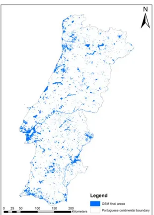
Exploratory analysis of OpenStreetMap for land use classification

O texto busca refletir sobre a emergência daquele que é considerado o sentido moderno do conceito de Revolução, tendo como objetivo a discussão da trajetória que passa do

The proposed model of two professionalism models (Evetts, 2010, p.130): organ- isational-based professionalism and occupational-based professionalism in knowledge societies is

Tendo em conta o Projeto Pedagógico “Uma Viagem no Verde” e o Projeto Curricular da sala dos 4 anos “A viajar o mundo vou descobrir…” pretende-se que cada criança

The results obtained from this work, indicate that for Large and Medium Offices the NV ventilation was effective until at least 3H, while for Long Office it was shown that

Se os computadores e a internet são, hoje em dia, considerados ferramentas fundamentais para o estudo, o desempenho de uma profissão e mesmo para o exercício

No corpo do nosso artigo, fizemos notar não apenas que o célebre momento da peripécia em Frei Luís de Sousa (Acto II, cena XV, aliás ecoando em réplicas trocadas entre

We compare a fuzzy-inference method with two other computational intelligence methods, decision trees and neural networks, using a case study of land cover classification from

Os dois tipos de jambu estudados mostraram-se também fonte de compostos fenólicos totais com valores de 360,21 (mg/L) para o jambu convencional e 396,89 (mg/L) para o