Interaction of Noncommutative Solitons with Defects
Alidad Askari∗ and Kurosh Javidan
Department of Physics, Ferdowsi University of Mashhad 91775-1436 Mashhad Iran [email protected], [email protected]
(Received on 5 November, 2008)
Interaction of solitons of noncommutative sine-Gordon model with potentials is studied by including a po-tential through one of the soliton parameters. The bahaviour of non commutative solitons during the interaction are compared with commutative solitons and the differences are explained.
Keywords: Solitons; Nonlinear field theory; Noncommutative field theory
1. INTRODUCTION
Noncommutative field theories are interesting subjects in the most of the branches of sciences. It has attracted a great deal of attentions in recent years; however the development of noncommutative field theory has a long history. There are many of new works in the construction of Noncommutative solitons and instantons [1, 2].
It has been shown that 1+1 noncommutative space-time where the time is necessarily a noncommutative coordinate, leads to nonunitarity and also lacks the causality [3, 4]. These difficulties can be solved by using a suitable two-dimensional Euclidean model. Integrebility of the model is another seri-ous problem. After introducing the noncommutative case for the field theory, obtained by considering the replacement of the usual product of the fields by their *-product, some of the models are still integrable while another are not. This problem has been removed by several methods, for example redefining the field equations by using a suitable generalization of the zero-curvature technique [5].
Here we focus on a suitable version of noncommutative sine-Gordon (NCSG) model. NCSG model is intuitively de-fined as a model which reduces to the ordinary one when non commutation parameter goes to zero. But the general-ization of noncommutative version of the field theories is not unique, as one may construct different noncommutative equa-tions of motion which reduces to the same expression when the noncommutative parameter vanishes. As we have men-tioned before, a successful generalization of two-dimensional integrable systems at the level of equations of motion can be performed by using the zero-curvature method.
An interesting question is how noncommutativity could af-fect on the dynamics of the soliton during the interaction with a potential, which we will try to investigate the features of this question.
This manuscript is organized as follows. In the next section we will describe a suitable NCSG system and its solitonic so-lutions. A model for soliton-potential system is explained in section3. Interaction of non commutative solitons with a po-tential barrier will be discussed in section 4. The behaviour of a non commutative soliton during the interaction with a po-tential well is explained in section 5 and Section 6 contains
∗Present address: Hormozgan university Po.Box 3995 Bandar Abbas Iran
conclusion and remarks.
2. NONCOMMUTATIVE SINE-GORDON MODEL
The Lagrangian of the sine-Gordon model is
L
=12∂µφ∂
µφ−λ(1−cosφ) (1)
The usual noncommutative case of the model is obtained by changing the ordinary product of the fields with the *-product in the lagrangian (1) and consequently in the equation of mo-tion. The result has causality problem and also it is not inte-grable. The first problem can be solved by using Euclidean space with the following components:
Z=√1 2
¡
x0+ix1¢,Z¯=√1 2
¡
x0−ix1¢ (2)
non commutativity is encoded in the relation[Z,Z¯] =θwhere
θis a real parameter. With the above variables (1) reads
L
=∂φ∂φ¯ +2λ(1−cosφ) (3)where∂=∂∂Z and ¯∂=∂∂Z¯.
Integrability problem can be solved by using the bicom-plex implemented method in noncommutative geometry for the NCSG model, which has been fully demonstrated in [6]. The results are unexpected and differ from the ’natural’ gen-eralized NCSG model. Indeed a system of two coupled equa-tions of motion are produced which are describe the evolution of the field
¯ ∂
µ e
iφ 2
∗ ∗∂e
−iφ 2
∗ +e
−iφ 2
∗ ∗∂e iφ
2
∗ 
=0
¯ ∂
µ e
−iφ 2
∗ ∗∂e iφ
2
∗ −e iφ 2
∗ ∗∂e
−iφ 2
∗ 
=iλsin∗φ
(4)
in which the *-product is defined as
(f∗g)(Z,Z¯) =exp
µθ
2
³
∂Z∂ξ¯−∂Z¯∂ξ ´
as∂∂φ¯ =λsinφ. The fieldφis a function of the noncommuta-tive parameterθand can be expanded in the orders ofθas
φ=
∞
∑
n=0φnθn (6)
Note that the dependency to the parameterθarises from the expansion (6) and also from the definition of *-product in the equations.
In the first order expansion ofφ, we haveφ=φ0+θφ1. For this situation equations (4) reduce to [6]
∂∂φ0¯ =λsinφ0
∂∂φ1¯ =λφ1cosφ0 (7) and the constraint equation
∂2φ0∂¯2φ0−¡
∂∂φ0¯ ¢2
=0 (8)
The solutions of the above equations are
φ
à soliton antisoliton
!
0 = (±)4arctan
µ exp
µ√
2λx1−√x¯1−ivx0
1−v2
¶¶
φ1= 1
cosh
µ√
2λx1√−x¯1−ivx0
1−v2 
(9) where ¯x1is the initial position of the soliton and ’v’ is its ve-locity. The fieldφ1is the first order correction generated by noncommutativity to the Euclidean one-soliton solution of the ordinary sine-Gordon model.
The topological charge for the noncommutative soliton can be defined as [6]
Q= 1 2π
Z ∞
−∞dx
1∂φ
∂x1 (10) It is interesting to know that the equations of motion (7) can be also derived from the action
S2= Z
d2x µ
1
2∂φ0∂φ0¯ +λ(1−cosφ0) +θ
¡
∂φ0∂φ1¯ +λφ1sinφ0¢ 
(11) The energy density is calculated from (11) as following
H
=12∂φ0 ¯
∂φ0−λ(1−cosφ0)−θ¡
∂φ0∂φ1¯ +λφ1sinφ0¢
(12) For the second order expansion of the φrespect to θwe have
φ=φ0+θφ1+θ2φ2 (13) With the following solitonic solution
φ soliton antisoliton
0 =±4arctan
µ exp
µ√
2λx1−√x¯1−ivx0
1−v2
¶¶
φ1= 1
cosh
µ√
2λx1−x¯1−ivx0
√
1−v2 
φ2(x1,x0) =− √2λ 2√1−v2tanh
µ√
2λx1−x¯1−ivx0
√ 1−v2
(14)
Here we will work with the first order expansion of the field with solution (9).
3. SOLITON-POTENTIAL SYSTEM
Scattering of commutative solitons (CS) from potentials (which generally come from the medium properties) have been studied in many papers by different methods. The ef-fects of medium disorders and impurities can be added to the equation of motion as perturbative terms [7, 8]. These effects also can be taken into account by making some parameters of the equation of motion to be function of space or time [9, 10]. We have added the potential through the parameterλwhich has been appeared in the solutions (9) and (14).λis set as
λ=
½
1+λ0 |x|<w 1 |x|>w
¾
(15) where parameter ’w’ describes the width of the potential re-gion. Clearly,λ<0 describes a potential well whileλ>0 creates a barrier. We can also use another types of localized functions for the parameterλ.
Equations (7) cannot be solved theoretically with a space dependent parameter like (15), so we have to solve it numer-ically. But we can use solution (9) as an initial conditions for solving (7), if soliton is located far from the center of the potential. We have performed simulations using 4th order Runge-Kutta method for time derivatives. Space derivatives have been expanded by using finite difference method. Grid spacing h=0.01, 0.02 and sometimes h=0.001 have been used in the simulations. Time step has been chosen as 14 of the space step ’h’. Simulations have been setup with fixed ary conditions and solitons have been kept far from the bound-aries during the simulation. We have controlled the results of simulations by checking the conserved quantities: total energy and topological charge, during the evolution.
4. INTERACTION OF A SOLITON WITH A BARRIER
First of all we need to know the shape of the potential. We can place a static soliton at different places and find the total energy of the soliton. This tells us what the potential is like as seen by the soliton [10, 11]. Fig. 1 shows the effective potential as seen by the soliton for an obstruction withλ0= 0.2. The dashed line shows the commutative case (θ=0)
and the solid line presents the situation for noncommutative soliton withθ=0.6. The energy of the commutative soliton in the absence of the obstruction isE0. The dash-dot line shows λ(x) +E0.
The total energy of a static commutative soliton in the ab-sence of potential is 6.1699 and the total energy of a non com-mutative static soliton withθ=0.6 is 6.1602. The energy of noncommutative soliton (NCS) is about 0.01 less than the en-ergy of a commutative soliton (CS) on top of the barrier of λ0=0.2. Therefore the effective mass of a NCS is less than the effective mass of a CS.
FIG. 1: Potential as seen by the soliton. Dashed line shows the po-tential for commutative soliton and solid line presents the situation for noncommutative soliton. The dash-dot line isλ(x) +E0
a critical velocityvc. In low velocitiesvi<vc, soliton reflects
back and reaches its initial place with final velocityvf ≈ −vi.
A soliton with an initial velocity vi>vc has enough energy
for climbing the barrier, and passing over the potential. The behaviour of a NCS can be investigated with direct sim-ulation of equations (7). The first equation of (7) is the equa-tion of moequa-tion of commutative sine-Gordon soliton. Therefore we can conclude that the general behaviour of a NCS is the same as the above description for a CS. The critical velocity can be found by sending a soliton with different initial speed and observing the final situation after the interaction (falling back or getting over the potential). Equations (7) also show that the critical velocity for a NCS is the same as the critical velocity of a commutative case.
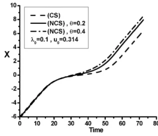
Figure 2 shows the trajectory of commutative and noncom-mutative solitons during the interaction with the barrier of λ0=0.1. Solitons move with a same velocity when they are far from the potential while CS travels ahead of the NCS. Fig. 1 shows that the NCS peak is located somewhere behind the CS peak after the interaction.
The difference between the energy of NCS and energy of CS decreases when their initial velocity increases. So the ve-locity of a NCS becomes bigger than the CS veve-locity during the interaction with the barrier. Therefore the peak of the NCS goes ahead of the CS peak. After the interaction solitons move with a same velocity while the peak of the NCS follows the NCS peak. Fig. 2 also shows that the distance between the peak of the solitons increases when the non commutation pa-rameterθincreases. Initial velocity in the above simulation has been selected very near to the critical velocity.
Figure 3 presents the trajectory of CS and NCS during the interaction with a barrier where the initial velocity is greater than the critical velocity. Figs. 2 and 3 clearly show that the interaction of NCS with a barrier is an elastic interaction sim-ilar to what we can observe for the interaction of a CS with
FIG. 2: Trajectory of a commutative soliton (dashed line) and non-commutative soliton with θ=0.2 (solid line) and another NCS withθ=0.4 (dash-dot line). The initial velocity of the solitons is v0=0.3045. The height of the barrier isλ0=0.1.
potential barrier. Also it can be concluded that a NCS makes a deeper interaction with a potential barrier as compared with a CS in a similar situation. The critical velocity can be found
FIG. 3: Interaction of CS and NCS with potential barrier. Initial velocity is greater that the critical velocity.
5. INTERACTION OF A SOLITON WITH A POTENTIAL WELL
Suppose a point particle moves toward a frictionless poten-tial well. It falls in the well with an increasing velocity and reaches the bottom of the well with its maximum speed. After that, it will climb the well with decreasing velocity and finally passes through the well. The final velocity of the particle after the interaction is equal to its initial velocity. But simulations show that the interaction of a commutative soliton with poten-tial well is not completely similar to the interaction of a point particle with a potential well [10, 11].
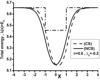
It is clear thatλ0<0 in the (15) corresponds to a potential well. Like the case of the barrier, we can find the shape of the potential as seen by the soliton with plotting the total energy of a static soliton placed in different positions (x). Fig. 4 shows the results for the obstruction with λ0=−0.2 andθ=0.6 (solid line). The dashed line in figure 5 presents the situation of a commutative soliton(θ=0)in the same potential well. Soliton-well interaction is a complicated situation. Suppose
FIG. 4: The potential wellλ0=−0.2 with as seen by the soliton.
The dashed line shows the potential for CS and solid line presents the situation for NCS. The dash-dot line isλ(x) +E0
a commutative soliton starts to move toward the well from an initial position far from the potential region. In this case again, there exists a critical velocity(vc)which separates two
different kinds of soliton behaviour. A Soliton with initial speed above the vc, transmits through the well and a soliton
with initial velocity lower than thevc falls into the well and
becomes trapped by the potential. As mentioned before, the critical velocity can be found by direct simulations with the first equation of (7) and this parameter is identical.
Consider a soliton with an initial velocity greater than the critical velocity. The soliton transmits through the well. The final energy and velocity of the soliton after the interaction is smaller than these quantities before the interaction. Fig. 5 presents the interaction of CS and NCS with the potential well ofλ0=−0.2. Initial velocity of the solitons isv0=0.2. Fig. 5
clearly shows that the NCS radiates more amount of energy as compared with the CS. Therefore the final velocity of a NCS after the interaction is smaller than the final velocity of a CS in the same situation. Fig. 5 also shows that the final velocity of the NCS decreases when the noncommutative parametertheta increases.
FIG. 5: Interaction of CS and NCS with the potential well. The initial velocity is greater that the critical velocity.
Suppose a soliton with an initial velocity lower that the crit-ical velocity. Both CS and NCS become trapped in the well and oscillate there. In other words the situation for CS and NCS is almost the same. Fig. 6 shows this situation. In other words, the period of the oscillation is the same for a NCS and CS in the same potential well.
6. CONCLUSIONS AND REMARKS
Interaction of a non commutative sine-Gordon soliton with defects was investigated. The non commutative soliton is con-structed in the first order of expansion,φ∗=φ0+θφ1.
A non commutative soliton interacts with a potential bar-rier almost elastically. At low velocities it reflects back and with a high velocity climbs the barrier and transmits over the potential. Energy exchanges between the soliton and the bar-rier during the interaction. The final speed of the soliton after the interaction is almost equal to its initial speed with a very good approximation. There exists a critical velocity which separates these two kinds of trajectories.
But for the case of soliton-well interaction, we observe in-teresting effects. A high speed soliton passes through the po-tential well and a low speed soliton becomes trapped in the well and oscillates there. In both situations the soliton emits energy, so its energy decreases in time to a stable state. In the
noncommutative case the Soliton radiates more energy than the same soliton in commutative space.
It can be concluded that a non commutative soliton has a deeper interaction with defects. This means that the effective potential in the non commutative case is greater than the ef-fective potential in the commutative plane. Therefore the final velocity of the soliton after the interaction in the non commu-tative case is lower than the final velocity in a commucommu-tative model. We expected to find an energy exchange between the parts of the field in the non commutative soliton. Some very interesting results can be related to such energy exchange. But we could not find an energy exchange between the two parts of the field in non commutative soliton in our simulations. It is because of the smallness of non commutative parameterθ. It is very interesting to study the phenomena with a suitable col-lective coordinate system. But constructing such coordinates needs more advanced investigations.
[1] N. Nekrasov, A. Shwarz, Comm. Math. Phys.198, 689 (1998). [2] R. GopaKumar, S. Minwalla, and A. Frominger, JHEP0005,
020 (2000).
[3] N. Seiberg, L. Susskind, and N. Toumbas, JHEP0006, 044 (2000).
[4] J. Gomis, T. Mehen, Nucl. Phys. B591, 265 (2000).
[5] L. D. Fedeev, L. A. Takhtajan,Hamiltonian methods in the the-ory of solitons. Springer, Berlin (1987)
[6] M. T. Grisaru, S. Penati, Nucl. Phys. B.655, (2003) [hep-th / 0112246]
[7] Y. S. Kivshar, S. Fei, and L. Vasquez, Phys. Rev. Lett67, 1177 (1991).
[8] Z. Fei, Y. S. Kivshar, and L. Vasquez, Phys. Rev. A46, 5214 (1992).
[9] B. Piette, W. J. Zakrzewski, [hep-th/0611040]
[10] B. Piette, W. J. Zakrzewski, and J. Brand, J. Phys. A: Math. Gen.38, 10403 (2005).