*e-mail: [email protected]
Article presented at the Congress SAE Fatigue 2004, São Paulo - SP, June/2004
Residual Analysis Applied to S-N Data of a Surface Rolled Cast Iron
Omar Malufa*, Marcelo Tadeu Milana, Dirceu Spinellia, Mariano E. Martínezb a
Departmentt of Materials, Aeronautics and Automotive Engineering
b
Department of Structures Engineering School of São Carlos, University of São Paulo,
13566-590 São Carlos - SP, Brazil
Received: August 11, 2004; Revised: April 5, 2005
Surface rolling is a process extensively employed in the manufacture of ductile cast iron crankshafts, specifically in regions containing stress concentrators with the main aim to enhance fatigue strength. Such process hardens and introduces compressive residual stresses to the surface as a result of controlled strains, reducing cyclic tensile stresses near the surface of the part. The main purpose of this work was to apply the residual analysis to check the suitability of the S-N approach to describe the fatigue properties of a surface rolled cast iron. The analysis procedure proved to be very efficient and easy to implement and it can be applied in the verification of any other statistical model used to describe fatigue behavior. Results show that the conventional S-N methodology is able to model the high cycle fatigue behavior of surface rolled notch testpieces of a pearlitic ductile cast iron submitted to rotating bending fatigue tests.
Keywords:surface rolling, fatigue, residual stress, statistical model, residual analysis
1. Introduction
Ductile cast iron is produced through the addition of a metallic alloy containing Fe-Si-Mg to a base cast iron in order to produce nodular graphite, instead of flake graphite as found in grey cast irons1.
This process allows the manufacturing of materials with improved mechanical strength and ductility which are extensively used in the fabrication of mechanical parts such as crankshafts. Strength and ductility are dependent on the matrix microstructure2. Depending on
the chemical composition and heat treating, the matrix can be either ferritic, pearlitic, ferritic-pearlitic, bainitic, martensitic or austenitic3.
Size and distribution of the graphite nodules in the matrix are also important to the mechanical properties4.
The fatigue strength of a cast part depends not only on the microstructure and chemical composition, but also on the surface finishing and geometry of the part. Dimension gradients and notches are stress concentrators which are prone to fatigue crack nucleation and if they cannot be avoided in the design of part, they must undergo special treatments5. For example, in order to eliminate sharp ends
in automotive crankshafts, notches are machined with a minimum radius which is subsequently surface rolled6. The main aim of such
procedure is to reduce notch sensitivity in these regions and thus reducing fatigue crack nucleation probability in critical regions of mechanical parts7.
Although statistical models are largely used in fatigue data analy-sis, a verification of the suitability of the model is not always checked. The main purpose of this work was to apply the residual analysis to check the suitability of the conventional S-N approach to describe the fatigue properties of a surface rolled cast iron. Additionally, the authors expect that this paper is capable of introducing a step-by-step procedure for the implementation of the residual analysis to any statistically significant model.
2. Residual Analysis
2.1. S-N curve
The most usual way of representing fatigue results is the S-N curve, where S is the applied stress amplitude or the maximum
ap-plied stress and N is the number of cycles for failure. In this curve, N values are plotted on the abscissa axis and S values are plotted on the ordinate axis8. Generally, these results are plotted in bi-logarithmic
scale resulting in a curve which can be expressed by:
log(N) = A + Blog(S) (1)
where A and B are the regression coefficients to be determined. Although Equation 1 is normally used to model fatigue life, the number of cycles for failure, N, may depend not only on S values but also on other independent variables which can be statistically significant. In the particular case of surface rolled parts, the presence of surface compressive residual stresses can potentially affect the model. Cyclic loading may cause residual stress relaxation which is closely related to the level of applied stresses. Experimental work and theoretical models have shown that higher applied loads are likely to cause both higher relaxation rate and higher relaxation levels9,10. Thus,
there could be non-linear relationships such as quadratic and exponen-tial that would better describe the fatigue properties of surface rolled parts. In this sense, these considerations raise a few questions:
1. How to identify that the assumed independent variables of the model are statistically significant?
2. How to check that the proposed model is adequate to describe the fatigue behavior of the material?
Normally, the answer to these questions is obtained by using a residual analysis of the statistical model.
2.2. Statistical model
A statistical model is a mathematic model which contains a random error with a specific probability distribution. Usually, this model is used to predict the value of one of the variables when the other is known, under specific conditions11. In a statistical model, two
The independent variable, X, is considered free of errors because X is not a random variable.
There is a linear relationship between Y e X and the statistical model that relates Yi to Xi is given by:
Yi = A + B Xi + εi (2)
for i =1, …, n, where n is the number of observations.
In Equation 2, A and B are unknown constants to be estimated and they are called parameters of the regression model. εi is a random value, denominated random error. The value of εi for any observa-tion will depend on both a possible error of measurement and other variables different from Xi that were not measured that could affect Yi. The values of εi are random variables, assuming the following assumptions:
1. The average of εi values is equal to zero and its variance, σ2, is
unknown and constant for 1 ≤ i ≤ n.
2. εi values are not correlated.
3. The distribution of εi values is normal for 1 ≤ i ≤ n.
Second and third assumptions imply that εi values are mutually independent.
The regression line is, in general, unknown and therefore must be estimated through the sampling data. In the particular case where the regression of Y in relation to X is linear, the best fit line can be written as:
^
Yi = A + ^ Bx^ i (3)
where the symbol “caret” (^) denotes estimate (estimator), A and^ andand B ^ are determined by the least squares method and Y^i are the estimated values of YYi using Equation 3 and the differences between Yi and Y^i shall be minimum. Generally, these differences are known as residu-Generally, these differences are known as residu-als, i.e., errors associated to the predicted values of Yi corresponding to each Xi value and which can be calculated through the following expression:
^
ei = Yi – Y^i (4)
2.3. Verifying the adequacy of the linear model
One of the most important tools for the verification of the ad-equacy of a regression model is the residual analysis. Values obtained by Equation 4 are the base for this procedure13. In this analysis, it is
possible to check if the assumptions about the residuals of the model, given by Equation 1, are satisfied, i.e., to verify that equal variance, normality and independence are accomplished. The validity of such assumptions can be verified through graphical analysis.
In order to evaluate the assumption of equal variance, in general, the residuals are plotted against the estimated Y. This assumption will ^ be valid if the dispersion of residuals in such plot does not reveal any obvious pattern. In Figure 1, a valid graph to accept the suitability of the model is presented, where the residuals are randomly distributed with equal variance.
If a funnel shape graph is obtained (Figure 2), the variance increases, indicating non - constancy. When inconstancy is found, data in both axes should be plotted in a logarithmic scale in order to stabilize the variance.
The verification of residuals normality can also be analysed by plots, such as normal score and normal probability graphs. In these graphs, the assumption of normality is valid if the points in the graph are localized approximately along a straight line. However, in case of doubt, the linearity can be confirmed using a statistical test of normal-ity, such as the one proposed by Shapiro and Francia14.
The assumption of independence can be checked by a graph of residuals against time (order of data collection). If the residuals are randomly distributed along the time axis, the independence
assump-tion will be valid. On the other hand, if a cyclic pattern, for example, is present in the graph, it means that the data is not independent.
Another tool to analyse the suitability of the regression model is the coefficient of determination, R2. However, the residual analysis
must always be performed because it allows identifying the lack of correlation and indicates possible adequate models. The coefficient of determination is given by:
( )
( )
R
Y Y Y Y
i i
n i i
n
2
2 1
2 1
=
-= =
r
t r
!
!
(5)
where the symbol “overbar” ( - ) denotes average.
Once the suitability of the model given by Equation 2 is checked, it is possible to infer and create prediction intervals more reliably and hence to estimate fatigue life (or stress levels for a given life) with greater confidence.Within the range of experimental points, the prediction interval 100(1 – α)% for a particular variable Yo is estimated by:
( )
Y t
n S
X X 1
/
xx e
0 2
2
! a { +
-t t r (6)
For points outside the testing interval, the prediction interval is given by:
( )
Y t
n S
X X
1 1
/
xx e
0 2
2
! a { + +
-t t r (7)
where,
^
Y0 = A + ^ Bx^ e (8)
Residuals
Estimated Values 0
Figure 1. Example of a graph of residuals (e^i) against the estimated values
(Y^i) when the regression model is adequate.
Residuals
Estimated Values 0
Figure 2. Example of a graph of residuals (e^i) against the estimated values
( )
n Y Y
2 i i i
n
2
2 1
{=
-= t
t
!
(9)
( ) /
Sxx n Xi X n
i n
i i
n
2 1
2 1
=
-= =
)
!
!
3 (10)and Xe is a specific value of X outside the interval of observed val-ues, α is the significance level, t(α/2) is determined from a t Student distribution with n-2 degrees of freedom and j^
is √
_
(j^2).
3. Experimental Procedures
In this work, bending rotating high cycle fatigue tests were performed in surface rolled notch testpieces of ductile cast irons. The matrix microstructure presented on average 85% of pearlite and 15% of ferrite; more than 80% of the graphite nodules were type I and II, according to ASTM A2474. Average results of tensile
tests indicated that the material is a 100-70-03 class material, accord-ing to ASTM A53615. All tests were performed in room temperature
and in as-cast condition. Average chemical composition is presented in Table 1.
For the bending rotating fatigue tests, notched testpieces were manufactured according to ASTM E46616, as seen in Figure 3. The
notch was surface rolled prior to fatigue testing. Bending rotating fatigue tests were performed according to ASTM E46817, under a
frequency of 92 Hz. Testpieces were considered non-failed when lives exceeded 107 cycles. The number of stress levels and the number
of testpieces tested at each stress level were determined according to ASTM E7398, in order to obtain a replication between 75% and
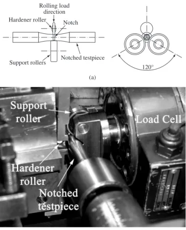
88%. The apparatus used for surface rolling the notches consists basically of 3 rollers disposed at 120° in relation to testpiece axis, as seen in Figure 4.
Rolling load was applied to the notch by a hardener roller which had a diameter of 15 mm, thickness of 5 mm and curvature radius of 1.3 mm. The other support rollers consisted of a 26 mm diameter sphere. The hardener roller was fixed to an apparatus used for surface rolling of crankshafts which was adapted for this work.
The apparatus was fixed to the tool post of a lathe and load was applied through the movement of the tool post perpendicularly to the testpiece axis which had both ends fixed to the lathe. Load was measured by a 10 kN load cell attached to the support rollers which were fixed to the base of the lathe. Load readings were acquired by a Transdutec-TMDE model digital reader. Testpiece notches were surface rolled under an applied load of 2.39 kN, frequency of 50 rpm and 250 revolutions.
4. Results and Discussion
Results of the fatigue tests are presented in Table 2. All data presented refer to fractured testpieces. Data analysis of the number of cycles for failure of the testpieces initiates with the verification of
Table 1. Average chemical analysis results (in weight %).
C Si Mn Cr Cu P S Mg
3.56 2.36 0.45 0.016 0.46 0.046 0.010 0.050
12.5
6.3 7.7
R 58
R 1.2
32
70
102
Figure 3. Notched testpiece for bending rotating fatigue tests.
Figure 4. Surface rolling apparatus: a) Schematic representation; b)
photo-graph of the equipment.
(b)
Rolling load direction Hardener roller Notch
Notched testpiece Support rollers
120°
(a)
Table 2. S and N values for surface rolled notch testpieces of ductile cast iron.
S (MPa) N (cycles for failure)
550 117900
550 148000
550 260700
550 264300
550 272100
525 222700
525 249500
525 312900
525 367400
525 1143900
500 2319900
500 1350000
500 2607300
500 1290100
500 695300
475 902800
475 4892000
475 1499900
Table 3. Regression coefficients of Equation 7 with their respective standard deviations s and to ratios.
Regression Coefficients s to
A = 54.599 7.079 7.71
B = - 17.992 2.611 - 6.89 the suitability of the model through the residual analysis. Estimated
values and the residuals are obtained by Equation 3 and Equation 4, respectively. In this work, all residual analysis calculations were performed using a statistics software package.
The graph of normal scores against the residuals was used to check if the normal distribution is attained (Figure 5). It is observed that the data results approximately in a straight line, indicating that the residuals of the model in principle follow a normal distribution. However, when the graph of residuals against estimated values is plot-ted (Figure 6), it is possible to observe a funnel shape which indicates an increase in variance. Therefore, the equal variance assumption is not attained and a modification of the model is necessary.
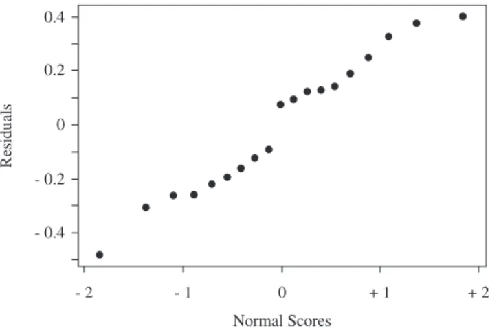
Therefore, a logarithmic conversion of both S and N data is performed to check if the assumptions of equal variance and nor-mality are obtained. As seen in Figure 7, the variance is constant. In Figure 8, the residuals can be approximately fitted by a straight line and the assumption of normality is attained. Hence, from the residual analysis it can be concluded that the stress level S is the only independent variable statistically significant and the model given by Equation 2 is adequate to describe the high cycle fatigue properties of surface rolled notch testpieces of the ductile cast iron of the present work. It is important to emphasize that if the assumptions of equal variance and normality were not attained even after the logarithmic transformation of both S and N scales, either the proposed model
would have to be described by a different mathematical function or an additional statistically significant independent variable would have to be included in the model.
Once the suitability of the model is checked, it is possible to obtain the linear relationship between logN and logS, as presented in Equation 11:
log(N) = 54.6 –18.0 log(S) (11)
This model shows a standard deviation (s) of 0.2632 and a coef-ficient of determination (R2) of 73.6% for n = 19 observations.
Ad-ditionally, Table 3 presents the regression coefficients of Equation 11 with their respective standard deviation s and to ratio.
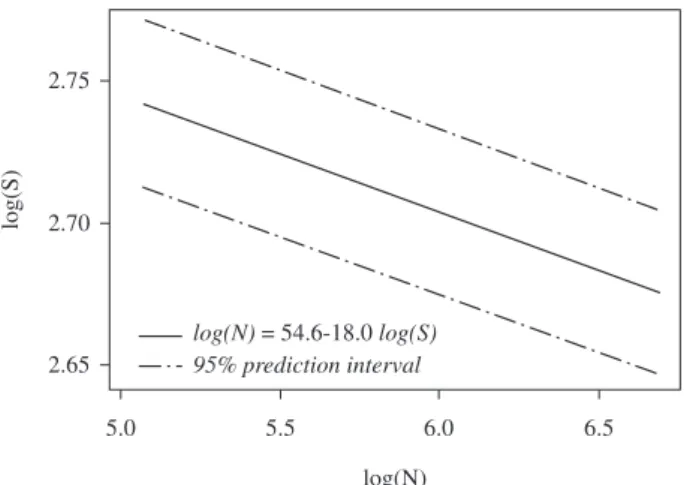
Figure 9 presents the S-N curve with a prediction interval of 95%. Observe that in this curve the independent variable S is plotted in the ordinate axis while the dependent variable N is presented in the abscissa as usually found in conventional S-N graphs8. Equation 11
Residuals
Normal Scores 0
0 1.106
2.106
- 1.106
- 2.106
- 2 - 1 + 1 + 2
Figure 5. Graph of residuals against normal scores values for rolled notch
testpieces.
Residuals
Estimated Values 0
0 1.106
2.106
- 1.106
- 2.106
3.106 1.106 2.106
Figure 6. Graph of residuals against estimated values for rolled notch
tes-tpieces.
Residuals
Normal Scores 0
0 0.2
0.4
- 0.2
- 0.4
+ 2 - 1
- 2 + 1
Residuals
Normal Scores 0
0.2 0.4
- 0.2
- 0.4
6.5 5.5 6.0
Figure 7. Graph of residuals against estimated values for rolled notch
test-pieces (after applying logarithmic scales).
Figure 8. Graph of residuals against normal scores for rolled notch testpieces
Figure 9. S-N curve and 95% prediction intervals for the surface rolled notch testpieces.
allows estimating accurately both the number of cycles for failure for a given applied stress level and the corresponding 95% predic-tion interval. However, in some cases it is necessary to determine the stress level at which failure will take place for a given number of cycles, in other words, it is necessary to obtain the endurance limit. According to Equation 11, for 2.106 cycles for example, the endurance
limit for the notch surface rolled testpieces of the ductile cast iron of the present work is approximately 483 MPa and the 95% prediction interval ranges from 459.8 MPa to 522.7 MPa.
5. Conclusions
A residual analysis procedure was successfully applied to analyze high cycle fatigue data of surface rolled notch testpieces of a pearlitic ductile cast iron tested under bending rotating fatigue. The procedure proved to be very simple and easy to implement and it can be applied to any statistical fatigue model. The residual analysis showed that the conventional bi-logarithmic model of S-N data is able to describe the fatigue properties of the cast iron, showing an endurance limit of approximately 483 MPa at 2.106 cycles calculated according to the
regression equation obtained from the model.
References
1. Labrecque C, Gagné M. Ductile iron: Fifty years of continuous develop-ment. Canadian Metallurgical Quarterly. 1998; 37(5):343-378.
2. QIT-Fer et Titane Incorporation. A Design Engineer’s Digest of Ductile Iron. 7th ed. Montreal: Rio Tinto Iron & Titanium, Inc., 1990.
3. Guesser WL, Hilário DG. Ferros fundidos nodulares perlíticos. Fundição
e Serviços. 2000; 11(95):46-55.
4. ASTM: A247-98. Standard Test Method for Evaluating the Microstructure of Graphite in Iron Castings. Annual Book of ASTM standards. West Conshohocken: American Society for Testing and Materials, 2001.
5. Maluf O. Influência do roleteamento no comportamento em fadiga de um
ferro fundido nodular perlítico. [MSc Thesis]. São Carlos: University of
São Paulo; 2002.
6. Daniewicz SR, Moore DH. Increasing the bending fatigue resistance of spur gear teeth using a presetting process. International Journal of
Fatigue. 1998; 20(7):537-542.
7. QIT-Fer et Titane Incorporation. Ductile Iron Data for Design Engineers. Montreal: Rio Tinto Iron & Titanium, Inc., 1990:75-80.
8. ASTM: E739-98. Standard Practice for Statistical Analysis of Linear or Linearized Stress-Life (S-N) and Strain-Life (ε-N) Fatigue Data. Ameri-can Society for Testing and Materials, Annual Book of ASTM standards, vol.03.01, Philadelphia, 2000.
9. Farrahi GH, Lebrun JL, Couratin D. Effect of shot peening on residual-stress and fatigue life of a spring steel. Fatigue and Fracture of
Engineer-ing Materials and Structures. 1995; 18(2):211-220.
10. Zhuang WZ, Halford GR. Investigation of residual stress relaxation under cyclic load. International Journal of Fatigue. 2001; 23:S31-S37, 2001 11. Martínez ME. Desenvolvimento de um modelo estatístico para aplicação
no estudo de fadiga em emendas dentadas de madeira. [PhD Thseis]. São
Carlos: University of São Paulo; 2001.
12. Chatterjee S, Price B. Regression Analysis by example. New York: John Wiley & Sons, Inc., 1977.
13. Draper NR, Smith H. Applied Regression Analysis. New York: John Wiley & Sons, Inc., 1998.
14. Shapiro SS, Francia RS. Approximate analysis of variance test for normality. Journal of the American Statistical Association. 1972; 67(337):215-223.
15. ASTM: A536-98. Standard Specification For Ductile Iron Castings. American Society for Testing and Materials, Annual Book of ASTM
standards, vol.01.02, Philadelphia, 2000.
16. ASTM: E466-96. Standard Practice for Conducting Force Controlled Constant Amplitude Axial Fatigue Tests of Metallic Materials. Annual
Book of ASTM standards. West Conshohocken: American Society for
Testing and Materials, 2000.
17. ASTM: E468-98. Standard Practice for Presentation of Constant Am-plitude Fatigue Tests Results for Metallic Materials. Annual Book of
ASTM standards. West Conshohocken: American Society for Testing
and Materials, 2000.
log(N)
log(N) = 54.6-18.0 log(S) 95% prediction interval
log(S)
2.75
2.70
2.65
6.5 5.5