INTRODUCTION
Thermal conductivity, thermal diffusivity and specific heat are the three most important physical properties of a material that are needed for heat transfer calculations. The equation relating these properties is given by:
a
ρ
= k
c p (A)
where: a = thermal diffusivity (m2/s), k = thermal conductivity
(W/m.K), ρ = bulk density (kg/m3) and c
p = specific heat
(J/kg.K).
Thermal conductivity is the property that determines the working temperature levels of a material, and it is an important parameter in problems involving steady state heat transfer. However, it is one of the physical quantities whose measurement is very difficult and it requires high precision in
Numerical and experimental determination of the minimum and maximum
measuring times for the hot wire parallel technique
(Determinação numérica e experimental dos tempos máximo e mínimo na
técnica de fio quente paralelo)
W. N. dos Santos, R. Gregório
Departamento de Engenharia de Materiais - DEMa Universidade Federal de S. Carlos - UFSCar
Rod. Washington Luiz, km 235, C.P. 676, S. Carlos, SP, 13565-905 [email protected]
Abstract
The hot wire technique is considered to be an effective and accurate means of determining the thermal conductivity of ceramic materials. However, specifically for materials of high thermal diffusivity, the appropriate time interval to be considered in calculations is a decisive factor for getting accurate and consistent results. In this work, a numerical simulation model is proposed with the aim of determining the minimum and maximum measuring time for the hot wire parallel technique. The temperature profile generated by this model is in excellent agreement with that one experimentally obtained by this technique, where thermal conductivity, thermal diffusivity and specific heat are simultaneously determined from the same experimental temperature transient. Eighteen different specimens of refractory materials and polymers, with thermal diffusivities ranging from 1x10⁻⁷ to 70x10-7 m2/s, in shape of rectangular
parallelepipeds, and with different dimensions were employed in the experimental programme. An empirical equation relating minimum and maximum measuring times and the thermal diffusivity of the sample is also obtained.
Keywords: hot wire technique, numerical simulation model, minimum and maximum measuring time, thermal properties, refractories.
Resumo
O método do fio quente é considerado como uma técnica precisa na determinação da condutividade térmica de materiais cerâmicos. Todavia, especificamente para materiais de alta difusividade térmica, o intervalo de tempo apropriado a ser considerado nos cálculos é um fator decisivo na obtenção de resultados precisos e consistentes. Neste trabalho, um modelo de simulação numérica é proposto com o objetivo de se determinar os tempos mínimo e máximo de medida na técnica de fio quente paralelo. O perfil de temperatura gerado por este modelo está em excelente concordância com aquele determinado experimentalmente por esta técnica, onde a condutividade térmica, a difusividade térmica e o calor específico são simultaneamente determinados a partir do mesmo transiente experimental de temperatura. Dezoito amostras diferentes de refratários e polímeros, com difusividades térmicas variando de 1x10⁻⁷
a 70x10-7 m2/s, na forma de paralelepípedos retangulares, e com diferentes dimensões foram utilizadas no programa experimental.
the determination of the parameters involved in its calculations. Nowadays, several techniques are available for the determination of thermal conductivities of different materials. However, for refractory materials the hot wire technique is a suitable method and it was specifically developed for this kind of material. Four variations of the hot wire method are known [1]: hot wire standard technique, hot wire resistance technique, two-thermocouple technique and the hot wire parallel technique. The basic theoretical model is the same, and the basic difference among these variations lies in the temperature measurement procedure. Two pieces are required whatever is the variation to be used. In this work, the hot wire parallel technique is employed in the experimental programme.
The hot wire parallel technique is an absolute, non-steady state and direct method, and therefore it makes the use of standards unnecessary. The hot wire method was described by Schieirmacher in 1888 [2], and its first practical application was reported in 1949 by Van der Held and Van Drunen [3], in the determination of the thermal conductivity of liquids. However, it was Haupin [4] who in 1960 first used this method to measure the thermal conductivity of ceramic materials. Nowadays, the hot wire method is considered an effective and accurate means of determining the thermal conductivity of ceramic materials. In addition, with the hot wire technique the concept of “mean temperature” between hot and cold face of a sample in thermal conductivity calculations is eliminated, since the measurement is carried out at a fixed temperature [5]. The temperature gradient across the sample is very low, and this is another virtue of this technique, since an ideal method for measuring the thermal conductivity would have to be capable of measuring this property across a zero temperature gradient throughout the sample.
In the mathematical formulation of the method, the hot wire is assumed to be an ideal, infinitely thin and long heat source which is in an infinite surrounding material, whose thermal conductivity is to be determined. This assumption implies that the temperature transient that is picked up by the thermocouple joint, at the measuring point, during the experiment cannot be altered by the fact that the actual sample has finite dimensions. These considerations imply some restrictions in the applicability of the hot wire technique in terms of possible sample sizes and thermal conductivity allowable ranges.
Applying a constant electric current through the wire, a constant amount of heat per unit time and unit length is released by the wire and propagates throughout the material. In practice, the theoretical infinite linear source is approached by a thin electric resistance and the infinite solid is replaced by a finite sample. In the plot of the recorded temperature at the measuring point as a function of time, the early part of the curve must be neglected in calculations because of the non-vanishing contact resistance between wire and sample, and the heat capacity of the wire. Also, a limit to the maximum measuring time has to be considered in the calculations because of the finite sample size. When heat reaches the outer surface of the sample, heat exchanges between the sample and the environment make the theoretical model no longer valid. The intermediate region of the curve where the theoretical model is valid defines the time limits to be considered in any measurement. So, the correct determination of the minimum and maximum times to be considered in the calculations is of fundamental importance for getting accurate and consistent results.
Applying a constant electric current throughout the wire, and recording the temperature increase at the measuring point, the thermal conductivity is calculated according to the following equation [6]:
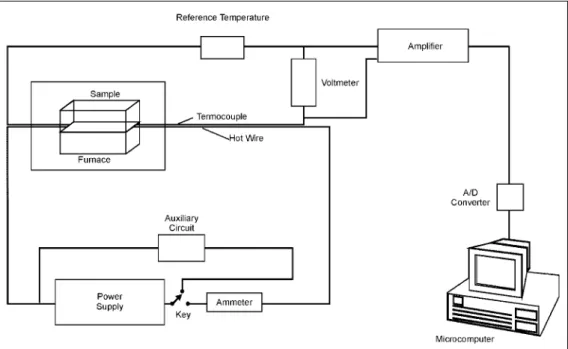
Figure 1: Schematic of hot wire parallel equipment.
(B)
where: k = thermal conductivity of the material (W/m.K), q’ = linear power density (W/m), ρ = material bulk density (kg/m3), c
p = specific heat of the material (J/kg.K), r = distance
between hot wire and thermocouple (m), t = elapsed time after beginning of heat release (s), T(t) = temperature rise registered by the thermocouple related to the initial reference temperature (K), and -Ei (-x) is the exponential integral function.
The calculations, starting from the recorded temperature transient in the sample are carried out by using a non-linear least squares fitting method [7]. Both thermal conductivity and specific heat in equation B are fitted in order to obtain the best possible approximation between the thermal transient experimentally registered and that one predicted by the theoretical model. In this case, these two thermal properties, thermal conductivity and specific heat are simultaneously determined from the same experimental transient, and with the knowledge of the density, the thermal diffusivity is then calculated using equation A. So, using the same apparatus it is possible to determine these three thermal properties in the same experiment.
The schematic diagram of the apparatus used in this work, as shown in Fig. 1, is fully automatic, and the transient of temperature detected by the thermocouple is recorded and processed by a computer via an analog-to-digital converter using a software specially written for this purpose.
THE SIMULATION MODEL
Since the method assumes an infinitely long and thin heat source, the heat conduction inside the specimen is of a radial nature [8, 9]. It is assumed that the solid is composed of N
concentric individual layers with radii ri measured from the center of the specimen where the hot wire is embedded. Fig. 2 illustrates this procedure.
An energy balance of the form of equation C may be defined for each region:
[Heat Flux in]i - [Heat Flux out]i =
[Rate of Internal Energy Change]i (C)
Then by applying balance equation C for each region, we derive equations D, E and F.
For i = 1:
(D)
For i = 2, 3,…, N-1:
(E)
For i = N:
(F)
where: <Ti> = average temperature of the region i between times t and (t+∆t), t= time and ri = radius of the region i.
In order to facilitate the numerical calculations, a dimensionless transformation for position, time and temperature, as shown in equations G, H and I is introduced.
(G)
(H)
(I)
where: Lref = any reference linear dimension (distance hot wire-thermocouple, for example), Trt = room temperature, Tref = any reference temperature (water vaporization temperature, for example),
r
i*= dimensionless radius of the region i, τ= dimensionless time and θ
i= dimensionless
temperature of the region i.
Taking as the dimensionless average temperature for each region, the arithmetic mean of the temperatures between
Figure 2: Annular cylindrical regions for the numerical analysis.
instants t and t+∆t, one can write equations J, K and L.
(J),
(K),
(L)
Combining equations D to L, and after some algebraic simplifications, the final result may be expressed in a matrix form given by equation M.
BKθK+1 = CKθK + D (M)
where: θ=column matrix of dimensionless temperatures, B and C=square matrices of dimensionless temperature coefficients terms, D=column matrix of dimensionless independent coefficients terms, and the superscripts K and K+1 refer to the times t and t+∆t.
The temperature profile generated by equation M at the measuring point Mp and at the edge of the sample can be used to determine the minimum and maximum measuring times to be considered in the calculations.
EXPERIMENTAL PROGRAMME
Eighteen different specimens of refractory materials and polymers in the shape of rectangular parallelepipeds with different dimensions were employed in the experimental
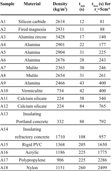
programme. Details of the samples are given in Table I. When it is possible to estimate the thermal conductivity and specific heat of the specimen to be tested, those values can be used as input data for the simulation model programme, in order to determine the adequate minimum and maximum measuring times for the hot wire parallel technique. However, if this estimate is not possible for any reason, an initial run of the hot wire technique will provide these values.
When the appropriate region of the temperature profile at the measuring point Mp is considered in the calculations, the resulting thermal property values are approximately constant, irrespective of the time interval considered inside this region. In this work, the criteria to determine the minimum and maximum measuring times were the increase by half a degree centigrade in the temperature at the measuring point and at the edge of the sample compared with the initial reference temperature. When calculations are carried out in this time interval, deviations among them are around 5% for all samples. Specific procedures for sample arrangements were described in several occasions [1, 10, 11]. In this work, the measuring point Mp was kept at 16 mm from the hot wire. Fig. 3 shows the samples arrangement.
Sample Material Density t
min tmax (s) for
(kg/m3) (s) r
s=5cm*
A1 Silicon carbide 2614 12 81
A2 Fired magnesia 2931 11 88
A3 Alumina zircon 3428 17 140
A4 Alumina 2901 22 177
A5 Alumina 2904 31 225
A6 Alumina 2676 28 243
A7 Mulite 2363 30 246
A8 Mulite 2654 31 261
A9 Alumina 2466 43 400
A10 Vermiculite 734 42 400
A11 Calcium silicate 224 58 540
A12 Calcium silicate 224 84 765
A13 Insulating
Portland concrete 332 88 792
A14 Insulating
refractory concrete 1710 108 957
A15 Rigid PVC 1368 205 1650
A16 Acrylic 1186 225 1775
A17 Polypropylene 906 225 2286
A18 Nylon 1151 260 2499
* rs = distance between hot wire and edge of specimen. Table I – Sample details.
[Tabela I - Detalhes sobre as amostras.]
Figure 3: Parallel hot wire technique. Experimental set-up.
RESULTS AND DISCUSSION
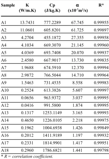
Measurements were carried out using the apparatus described in Fig. 1, and Table II shows the experimental results obtained for all samples.
Fig. 4 displays the temperature profile at the measuring point Mp during the measuring interval, evaluated with the simulation model, and experimentally determined with the hot wire parallel technique, for two selected samples: the sample with the highest thermal diffusivity, and that one with the lowest thermal diffusivity. Both plots show the perfect agreement between the results predicted by the simulation model and those ones experimentally determined by the hot wire method. This agreement assures the correct determination of the temperature profile at the measuring point and at the edge of the sample, and consequently the exact instant of the beginning of heat exchange between surface sample and environment, which defines the appropriate region of the thermal transient to be considered in the calculations.
Since the heat conduction inside the specimen is of a radial
Sample K Cp ααααα R*
(W/m.K) (J/kg.K) (x10-7m2/s)
A1 13.7431 777.2289 67.745 0.99955
A2 11.0601 605.8201 61.725 0.99897
A3 4.2704 455.1872 27.355 0.99958
A4 4.1034 669.3070 21.145 0.99960
A5 4.0369 693.7408 20.070 0.99937
A6 2.4580 667.9017 13.730 0.99835
A7 1.9688 674.5910 12.370 0.99994
A8 2.9872 766.5044 14.710 0.99964
A9 1.5463 731.4535 8.558 0.99983
A10 0.2524 613.3826 5.607 0.99997
A11 0.0656 963.9372 3.037 0.99995
A12 0.0416 991.5800 1.874 0.99995
A13 0.1317 1253.1149 3.165 0.99993
A14 0.4650 1226.0105 2.218 0.99975
A15 0.1962 1004.6938 1.426 0.99849
A16 0.2012 1411.9189 1.197 0.99932
A17 0.2331 1814.9901 1.417 0.99951
A18 0.2960 1786.6821 1.441 0.99798
* R = correlation coefficient.
Table II – Experimental results for the appropriate measuring time interval.
[Tabela II – Resultados experimentais para os adequados intervalos de tempo de medida.]
Figure 4: Temperature profile at measuring point.
[Figura 4: Perfil de temperatura no ponto de medida.]
nature and the samples tested have the parallelepiped shape, the heat exchange starts at points of the sample surface at a distance rs, the radius of the maximum cylinder inscribed in the experimental arrangement (Fig. 3) and having its central axis in the hot wire. After a relatively long elapsed time te, all the points on the surface will be exchanging heat with the environment, and then a stable temperature at the measuring point Mp is registered, as shown in Fig. 5. The value of the time te depends on the samples thermal diffusivity, relation between the parallelepiped dimensions, and the environmental conditions. In this work the criteria to determine minimum and maximum measuring times were the increase by half a degree centigrade at the measuring point and at the outer surface temperatures of the sample, in relation to the initial reference temperature. When calculations are carried out inside this time interval, the deviation in the thermal properties measurements is of approximately 5% for all samples. The correct determination of the minimum and maximum measuring times is a crucial and decisive task in the hot wire parallel
Figure 5: Temperature profile at measuring point: stable temperature after a long time.
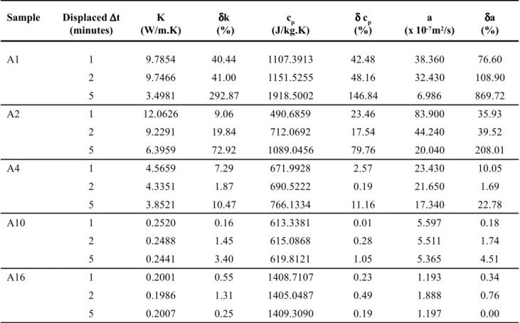
calculations, mainly for materials with high thermal diffusivities, and the higher the thermal diffusivity to be measured, the more critical its influence on the thermal properties measurements. Table III shows calculations taking into account the appropriate time interval [tmin, tmax] as stated in this work, and the results obtained when this same interval is displaced by 1, 2 and 5 minutes ahead for selected samples.
Sample Displaced ∆∆∆∆∆t K δδδδδk cp δδδδδ cp a δδδδδa
(minutes) (W/m.K) (%) (J/kg.K) (%) (x 10-7m2/s) (%)
A1 1 9.7854 40.44 1107.3913 42.48 38.360 76.60
2 9.7466 41.00 1151.5255 48.16 32.430 108.90
5 3.4981 292.87 1918.5002 146.84 6.986 869.72
A2 1 12.0626 9.06 490.6859 23.46 83.900 35.93
2 9.2291 19.84 712.0692 17.54 44.240 39.52
5 6.3959 72.92 1089.0456 79.76 20.040 208.01
A4 1 4.5659 7.29 671.9928 2.57 23.430 10.05
2 4.3351 1.87 690.5222 0.19 21.650 1.69
5 3.8521 10.47 766.1334 11.16 17.340 22.78
A10 1 0.2520 0.16 613.3381 0.01 5.597 0.18
2 0.2488 1.45 615.0868 0.28 5.511 1.74
5 0.2441 3.40 619.8121 1.05 5.365 4.51
A16 1 0.2001 0.55 1408.7107 0.23 1.193 0.34
2 0.1986 1.31 1405.0487 0.49 1.888 0.76
5 0.2007 0.25 1409.3090 0.19 1.197 0.00
Table III – Experimental results for displaced time intervals.
[Tabela III – Resultados experimentais para os intervalos de tempo deslocados.]
The deviation between those values increases as thermal diffusivity increases, showing the importance of these parameters for high thermal diffusivity materials. For sample A1 (silicon carbide brick) the displacement by only one minute in the measuring time interval is enough to introduce an error of 40% in the thermal conductivity, 42% in the specific heat and 77% in the thermal diffusivity.
Figure 6: Minimum measuring time as a function of the thermal diffusivity.
[Figura 6: Tempo mínimo de medida em função da difusividade térmica.]
Figure 7: Maximum measuring time as a function of the thermal diffusivity.
Figs. 6 and 7 display minimum and maximum measuring times as a function of the thermal diffusivity. Parameters tmin and tmax were fitted in order to provide a function relating these parameters and the thermal diffusivity. Correlation factor R2 shows the quality
of the fitting, indicating the validity of this procedure. Both equations should be used for an initial estimate of tmin and tmax.
CONCLUSIONS
A numerical simulation model is proposed to determine minimum and maximum measuring times in the hot wire parallel technique, with perfect agreement between the results predicted by this model and those ones obtained by the experimental method. The importance of the knowledge of the appropriate time interval to be considered in the calculations lies in the accuracy and reliability of the experimental results obtained. The influence of tmin and tmax in the hot wire parallel calculations is greatly increased as thermal diffusivity increases. With this simulation model it is also possible to determine minimum sample dimensions for a previous measuring time interval stated. The minimum and maximum measuring times were fitted to a power function and should be used for an initial estimate of tmin and tmax in the hot wire parallel technique.
ACKNOWLEDGEMENTS
The author wishes to thank FAPESP (Proc. 01/08225-4)
and CNPq (Proc. 300186/89-4 RN) for financial support. He also thanks IBAR-Industrias Brasileiras de Artigos Refratários for the specimens supplied.
REFERENCES
[1] W. N. dos Santos, J. S. Cintra Filho, Cerâmica 37, 252 (1991) 101.
[2] A. L. Schieirmacher, Wiedemann Ann Phys. 34 (1888) 38.
[3] E. F. M. Van Der Held, F. G. Van Drunen, Phy. 15, 10 (1949) 865.
[4] W. E. Haupin, Am. Ceram. Soc. Bull. 39, 3 (1960) 139. [5] W. R. Davis, F. Moore, A. M. Downs, Brit. Ceram. Trans. J. 79 (1980) 158.
[6] J. Boer, J. Butter, B. Grosskopf, P. Jeschke, Refractories J. 55 (1980) 22.
[7] J. P. Holman, Experimental Methods for Engineers, McGraw-Hill, New York (1971) 65.
[8] H. S. Carslaw, J. C. Jaeger, Conduction of Heat in Solids, Oxford University Press, Oxford (1959) 255.
[9] W. N. dos Santos, J. S. Cintra Junior, J. Eur. Ceram. Soc. 19, 16 (1999) 2951.
[10] P. R. E. Staff, Bull. Soc. Fr. Ceram. 126, 15 (l980) 15. [11] W. N. dos Santos, J. S. Cintra Junior, J. Eur. Ceram. Soc. 20, 11 (2000) 1871.