o
ABSTRACT: One issue the design team has to face in the process of building a new spacecraft, is to deine its mechanical and electrical architecture. The choice of where to place the spacecraft´s electronic equipment is a complex task, since it involves simultaneously many factors, such as the spacecraft´s required position of center of mass, moments of inertia, equipment heat dissipation, integration and servicing issues, among others. Since this is a multidisciplinary task, the early positioning of the spacecraft´s equipment is usually done “manually” by a group of system engineers, heavily based on their experience. It is an interactive process that takes time and hence, as soon as a feasible design is found, it becomes the baseline. This precludes a broader exploration of the design space, which may lead to a suboptimal solution, or worse to a design that will have to be modiied later. Recently, it has been shown the potential beneits of automating the process of spacecraft´s equipment layout using optimization techniques. In this paper, a prototype of an Excel® based tool for multidisciplinary spacecraft equipment layout conception is described. Provided the geometric dimensions, mass and heat dissipation of the equipment, and the available positioning area, the tool can automatically generate many possible trade-off solutions for the layout. It allows the user to set speciic equipment to speciic areas of positioning, and different combinations of objective functions can be used to drive the design. The features of the tool are shown in a simpliied three dimensional problem.
KEYWORDS: Layout optimization, Spacecraft, Conceptual design, Electronic equipment.
A Multidisciplinary Design Optimization
Tool for Spacecraft Equipment Layout
Conception
Valentino Lau1, Fabiano Luis de Sousa1, Roberto Luiz Galski1, Evandro Marconi Rocco1, José Carlos Becceneri1, Walter Abrahão dos Santos1, Sandra Aparecida Sandri1
INTRODUCTION
In the conceptual phase of the development of a new spacecrat, diferent candidate solutions for its electrical and mechanical architectures are assessed, in a search for one which would it the spacecrat mission, within the constraints of cost and schedule. It is in this phase that the main features of its subsystems are defined, and where the systemic and multidisciplinary character of the design process becomes more relevant to the deinition of its cost and performance.
he assessment of diferent solutions for the mechanical and electrical architecture includes the positioning of the spacecraft’s equipment over its structure panels, aiming at satisfying mechanical and electrical requirements or constraints. A target position for the system’s mass center, preference of moment of inertia in a given direction, minimization of electromagnetic interference, avoidance of high heat dissipation due to equipment being positioned close to another, and minimization of cabling are examples of such concerns. he early positioning of the spacecrat’s equipment is usually done “manually” by a group of system engineers, heavily based on their experience. Coupled to an analysis stage, where the system’s performance and constraints are veriied, the spacecrat’s equipment layout deinition is an interactive process that takes time and hence, as soon as a good feasible design is found, it becomes the baseline. his reduces the exploration of the design space, and increases the probability that better designs are missed. hus, increasing the creation of candidate solutions by numeric automatization of the
1. Instituto Nacional de Pesquisas Espaciais – São José dos Campos/SP – Brazil.
Author for correspondence: Valentino Lau | Instituto Nacional de Pesquisas Espaciais | Avenida dos Astronautas, 1.758, CEP: 12.227-010 – São José dos Campos/SP – Brazil | Email: [email protected]
search through the conceptual design space would increase the possibilities that better designs are found.
he works of Ferebbe Jr. and Powers (1987) and Ferebbe Jr. and Allen (1991) are probably the irsts to propose numerical optimization methods for automating the process of determining the layout of equipment during the conceptual phase of spacecrat design. In a series of works, Teng et al. (2001), Sun and Teng (2003), Zhang et al. (2008) and Teng et al. (2010), studied the eicacy of the approach when applied to a spinning telecommunication satellite, considering also the inluence of the application of diferent optimization methods. hese works have in common the focus on placing the equipment driven by the system’s mass properties (position of mass center and magnitude and direction of principal axis of inertia) requirements, subject to geometric constraints. In Jackson and Norgard (2002), thermal issues and minimization of wiring between equipment were introduced as objectives to be considered in the search for candidate solutions in the design space. hermal requirements are in fact one of the main drivers of the spacecrat layout design, and in the context of conceptual layout optimization they have been treated either by trying to meet requirements of equipment heat dissipation uniformity over the spacecrat’s structural panels (Jackson and Norgard, 2002; Hengeveld et al., 2011) or target temperatures on them (De Sousa et al., 2007). In the later work the problem was treated as fully multi-objective, that is, opposed to the usual approach of transforming it in mono-objective before optimization is performed, a set of trade-of solutions is the objective of the search. his provides more information about the design space, leaving for a posteriori analysis the choice of which solution will be implemented.
Coupling optimization algorithms with Computer Aided Design (CAD) and engineering analysis packages, provides an eicient way to tackle the spacecrat equipment layout problem, as highlighted in the works of Baier and Pühlhofer (2003), Pühlhofer et al. (2004) and Cuco (2011). In the later one, a new methodology was proposed to address the problem. he Cuco’s methodology (Cuco, 2011; Cuco et al., 2014) considers the main drivers commonly used to deine the equipment layout during the spacecrat’s conceptual design:
• he position of the system’s center of mass;
• he alignment and strength of the system’s main axis of inertia;
• Avoidance of concentration of high heat dissipation equipment over the satellite panels; and
• Equipment functional requirements.
The methodology of Cuco (2011), or different versions of it, may be implemented in different ways using commercial or custom made software. Cuco (2011) used modeFrontier
®
to couple Solidworks®
, Matlab®
, Excel®
and an executable written in C, for such purpose. The advantage of using a software such as modeFrontier®
as the core tool to implement the methodology is that, since it was specially developed to tackle optimization problems and act as an integrator of other CAD or Computer Aided Engineering (CAE) tools, it has readily available on its internal features different optimization algorithms and techniques to be used on the problem, and provides a user-friendly interface to integrate other tools and analyze the results. On the other hand, the user has limited or no access to changes on the workings of these tools, what may affect his/her ability to explore new ways of addressing the problem. In the context of a research tool for the exploration of different concepts and algorithms to address the spacecraft equipment layout optimization problem, Excel®
would provide a convenient alternative, since it can be used as a platform where new optimization algorithms can be embodied, as a calculator for engineering analysis, data storage, visualization of results, as well as an integrator of CAD and CAE tools. It also has the advantage of being known and be available largely in the engineering community.In the present paper, an Excel
®
based tool for spacecrat equipment layout is presented. Built using Cuco’s (2011) methodology as the optimization framework, it can provide the spacecrat design team an eicient and easy way to explore the layout conceptual design space. Excel®
was coupled to SolidWorks®
, which is used to calculate design parameters and as a graphical interface, where candidate layout conigurations can be visualized. The tool’s concept and early application tests were irst presented in the 22th International Congress of Mechanical Engineering (COBEM 2013) (De Sousa et al., 2013). he present paper is an updated version of the former. It introduces new features such as integrated decision making criteria for selection of solutions on the approximate Pareto frontier, additional objective functions and three-dimensional (3D) capability.o
SPACECRAFT EQUIPMENT LAYOUT
PUT AS AN OPTIMIZATION PROBLEM
The spacecraft’s layout problem can be tackled as a multidisciplinary multiobjective optimization problem and can be generally stated as:
Minimize
(1)
Subject to:
(2)
(3)
(4)
where fi is a vector of I objective functions, xj is a vector of J design variables, gk and hl are vectors of K and L inequality and equality constraints, respectively, and xjmin and xjmax
are the bottom and upper boundary constraints on the design variables.
he objective functions encode the design requirements for the spacecraft, such as a target position for its mass center, whereas the constraints deine the viable design space. For example, there must be no mechanical interference among the equipment. In the simpliied case study showed further in the text these points will be made clear.
The approach for the spacecraft equipment layout problem proposed by Cuco (2011) is used as the general framework to build the tool presented herein. The design variables are defined considering the faces of the panels where the equipment would be positioned and, over a given panel face, the local coordinate position of the equipment mass center being positioned on that panel. For a box-shaped equipment, the angle formed between the box edge and the panel axis is also a design variable. Hence, each equipment has 4 design variables: one index indicating in which panel’s face it is allocated, two local coordinates x and y of the position of the center of mass projected on the panel, and one orientation angle. For example, if there are 8 box-shaped equipment to be positioned and 2 panels available for positioning, there are 32 design variables for optimization. Design requirements
for the position of the system’s mass center, grouping of sets of equipment, avoidance of “hot spots” over the panels and, the alignment of the principal axis of inertia and the proportion of the principal moments of inertia are tackled by five objective functions, while geometric and functional requirements are take into account as constraints. In Cuco’s methodology, the result of the optimization is a set of candidate non-dominated solutions for the layout and its respective approximate Pareto frontier. The decision of which solution, or solutions, would be subject to a further analysis to become the baseline layout is left for the engineering team responsible for the layout design. The Cuco’s methodology framework embodies the basic aspects to be considered by any computational environment aimed at providing the system´s engineering team, a tool for the spacecraft´s equipment layout, during its conceptual design phase. It is flexible enough to accommodate design goals being treated either as objective functions or constraints.
Adding to Cuco´s work, the tool presented herein also incorporates decision making criteria to help the design team choose one or more candidate solutions for further evaluation, after the approximates Pareto set and Pareto frontier are returned.
For the general three-dimensional spacecrat layout problem, a practical tool must allow the exploration of any combination of equipment and positioning panel, as well as the possibility for the user to set a speciic combination of equipment/panel. For example, it may be desirable that some equipment is positioned over a panel of the spacecrat with the least incidence of Solar thermal radiation. Moreover, functional aspects may require that some equipment is ixed in a given position, or that a set of them are positioned close to each other. All these features are implemented in the tool presented here.
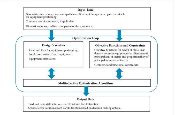
he main aspects considered for the conceptual spacecrat equipment layout are taken into account in the tool by 5 objective functions, which may be activated by the user independently. Mechanical interference between equipment is taken into account by constraints penalizing the objective functions, while parameterization of the design variables assures that the equipment remains inside the available positioning areas. he general optimization framework used for development of the tool is presented in Fig. 1.
Minimize:
(5)
(6)
(6.1)
(6.2)
(7)
(8)
(9)
Subject to:
(10)
(11)
(12)
(13) Input Data
G eometric dimensions, mass and spatial coordinates of the spacecraft panels available for equipment positioning.
Common sets of equipment, if applicable.
Dimensions, mass, and heat dissipation of the equipment.
Design Variables
Panel and Face for equipment positioning. Local coordinates of each equipment. Equipment orientation.
Objective Functions and Constraints
Objective functions for center of mass, heat density, common equipment set, alignment of principal axis of inertia and proportionallity of principal moments of inertia.
Geometric and functional constraints.
Multiobjective Optimization Algorithm
Output Data
Trade-off candidate solutions: Pareto set and Pareto frontier.
Set of selected solutions from Pareto frontier, based on decision making criteria.
Optimization Loop
o
f1 represents the goal of having the center of mass (CM) of the system, xi_CM_sys,as close as possible to a given target center of mass, xi_CM_target,. The parameters λi, which may assume zero or one value, are used to disable or enable the CM coordinate components. For example, if the CM longitudinal component of an spacecrat is less constrained than the other components, then only the lateral components could be enabled to drive optimization.
f2 is an object function devised to approximate the heat density over the spacecrat’s panels. his objective function is composed of two components. he irst one, f2Global, measures how far the layout is from an ideal condition of uniformly heat distribution over the entire spacecrat. Npanel is the number of panels; Nequi,p is the number of equipment installed in panel
p; Pi represents the heat dissipated by equipment i; Ap is the projected area of panel p; PTotal is the total heat dissipated; and ATotal is the total projected areas of the panels. he second component, f2,pLocal, evaluates the heat dissipated by the equipment
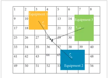
installed in panel p over discrete regions of this panel. he panel is divided in Ncell,p rectangular cells, each side of them with the size of rmin, which is the size of the smallest dimension, in contact with the panels, of all equipment divided by 2. ri,j
is the distance between the center of the ith equipment to the
center of jth cell, as seen in Fig. 2.
Minimizing f2,pLocal means that the standard deviation of the
quantity is minimized, that is, the combined inluence of all equipment over each panel cell would be the same.
his would avoid “hot spots” over the panel. he ratio r2 min/ATotal
is applied for scaling compatibility of these two components.
f3 represents the goal of minimizing the distance between equipment belonging to the same common set. We define here a common set, as a group of equipment that should be positioned near each other. di,j,k is the Euclidian distance between the geometric centers of equipments i and j belonging to a common set k, Nequi,k is the number of equipment in common set k and Nset is the number of common sets.
f4 measures the alignment of the principal axis of inertia to the spacecraft global coordinate system; αi are the angles formed between the i-axis of the principal inertia and global coordinate systems, as shown in Fig. 3; and αi_target is a given target angle. Analogously to λi in f1, the parameters
ρi, which are set to zero or one, are used to disable or enable angle components.
he goal of f5 is to achieve a given proportionality between the principal moments of inertia. vinertia is a vector which components are the tree principal moments of inertia, and vtarget is a given target vector, which components are positive values, that keep a desired proportion. For example, in a spacecrat controlled by spin, the longitudinal moment of inertia should be larger than lateral ones, say n times, while lateral moments of inertia could be of the same order. Setting the longitudinal component of vtargetto n and the lateral components to 1 would represent this proportion. he vector norm of the cross product gives the area of the parallelogram formed by these two vectors. If they
1 2 3
Equipment 1
Equipment 3
Equipment 2
r
1,28
r3,28
r
2,28
4 5 6 7 8
9 10 13 14
17 18 21 22
25 26 27 28 29 30
33 34 35 36 37 38 39 40
41 42 43 44 45 48
49 50 51 52 53 56
Figure 2. Representation of how the distance between the equipment and the panel’s cells is considered in the heuristic used to calculate ∫2
Local. Example with three equipment and 56
cells. Only distances for cell 28 are shown in the example, but all cells are considered when calculating the value of ∫2
Local.
ZPRINCIPAL
YPRINCIPAL
XPRINCIPAL
αZ
αX
αY
CM
ZGLOBAL
YGLOBAL
XGLOBAL
Iiθis an integer variable used to evaluate the rotation angle θ as indicated in Eq.16. The number of increments
Ndivision,i is defined by the user. The angle θ varies in the range 0°≤θ≤180°.
(16)
Vinter is the total volume of mechanical interference among equipment and structure. he equality constraint (Eq. 13) is treated as a penalty for the objective functions when it is violated, using an exterior penalty method (Vanderplaats, 2007) approach.
DESCRIPTION OF THE SPACECRAFT
EQUIPMENT LAYOUT CONCEPTUAL
DESIGN TOOL
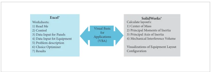
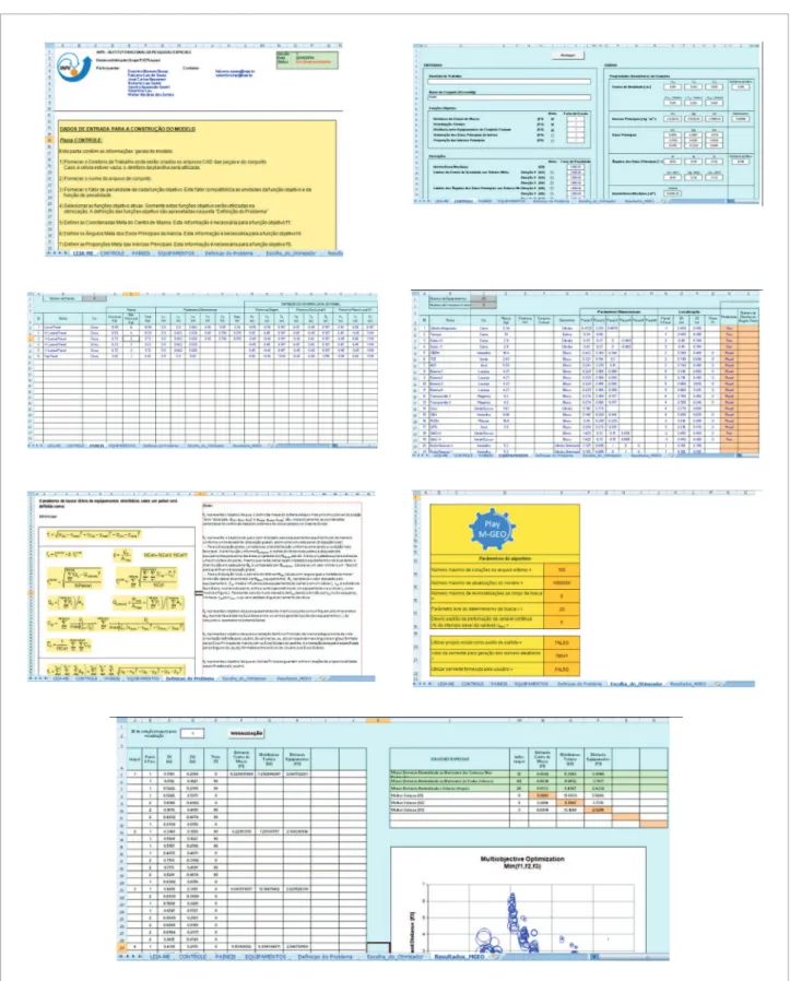
he main components of the optimal layout tool are presented in Fig. 5.
The Excel workbook consists of 7 worksheets and 3 main macros. From the Read Me worksheet, a description of all parameters used in this tool is presented. In the Control worksheet, parameters used to define and activate
L1
L2
e1 e2
B L
D2
CG H
D1
Y1
X1
Y1
X1 X2 Y2
θ θ
θ θ
Z1
Figure 4. Equipment position over the panel.
are aligned, what means that vinertia has the same proportion of vtarget, this area vanishes. On the other hand, if they are not aligned, a positive value is obtained. Normalization is used in order to keep f5 in the range of [0,1].
Tiface, s
i,l, si,2 and Ii
θ are the design variables.
he irst deines the panel and the face where equipment i is installed. his is an integer variable corresponding to the index of an element in a list that contains all available panel faces, coded as the panel ID number with a signal, positive for top face and negative for bottom face. he number of available faces, Nface,i, can vary for each equipment i, since constraints may be applied to restrict equipment installation.
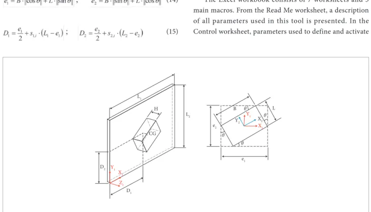
he next two variables deine the parameterized position of the geometric center of an equipment i over the panel. B, L and
H are the equipment dimensions, while L1 and L2 are the panel dimensions, and θ is the equipment rotation angle, as shown in Fig. 4. he distances e1 and e2 are deined in Eq.14, and the relationship between the parameterized variables and the local coordinates D1 and D2 are presented in Eq.15. he values of the parametric variables si,1 and si,2 can vary in the range [0, 1]. his parameterization guaranties that the boundaries of the equipment always lies inside the area of the panel.
(14)
o Worksheets:
1) Read Me 2) Control
3) Data Input for Panels 4) Data Input fot Equipment 5) Problem description 6) Choice Optimizer 7) Results
Visual Basic for Applications
(VBA)
Calculate layout’s: 1) Center of Mass
2) Principal Moments of Inertia 3) Principal Axis of Inertia 4) Mechanical Interference Volume
Visualizations of Equipment Layout Configuration
SolidWorks® Excel®
Figure 5. Main components of the spacecraft equipment layout tool.
objective functions and constraints are entered. A specific geometric configuration, defined in the Panels and Equipment worksheets, is built in SolidWorks
®
, which is launched by clicking a macro button inside the Control worksheet. All design parameters calculated inside SolidWorks®
, are returned to the Control worksheet. In the Panels worksheet the geometric characteristics of each panel available for equipment positioning is entered. In the present version of the layout tool only rectangular panels are modeled. In the Equipment worksheet, the mechanical and thermal characteristics of the equipment are entered, together with the information of what subsystem they belong. In the current version of the layout tool, rectangular, cylinder and sphere solid shapes can be used to simulate the equipment. The solids may be assigned with different colors. In this worksheet, it can also be entered values for the design variables. In the Problem Description worksheet, a brief description of the objective functions, constraints and design variables being considered in the optimization problem is provided. In the Choice of Optimizer worksheet, the optimization algorithm to be used is chosen and information concerning its operational, such as parameters and stopping criteria, is entered. The optimization process is initialized from this worksheet, by clicking a macro button representing an available optimization algorithm. This calls a routine that embodies the algorithm and links it to other routines that launch and control SolidWorks®
. Finally, in the Results worksheet, the approximate Pareto set and Pareto frontier obtained during the search are presented. Different types of graphs available in Excel®
may be used in order to showthe approximate Pareto frontier. For example, for problems with three objective functions, bubble or surface graphs may be used. In Fig. 6, screen prints of the seven worksheets are presented for illustration purposes.
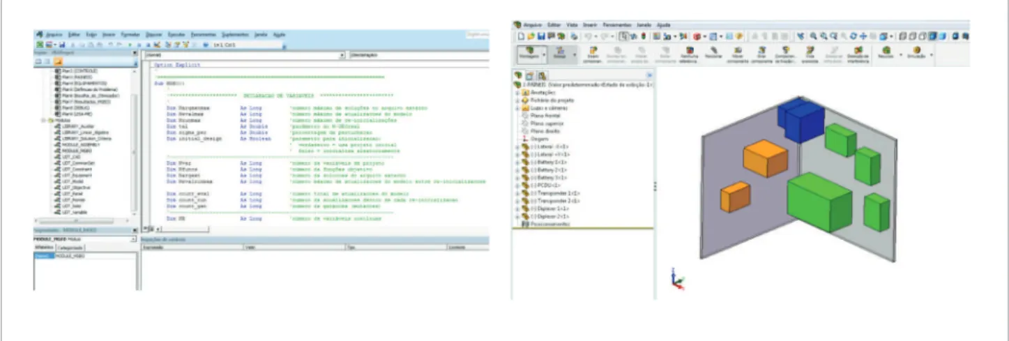
The macros for the optimization algorithms, objective functions and routines that link Excel
®
to SolidWorks®
are built using the VBA editor, in a modular approach, such that new optimization algorithms or objective functions can be added or removed from the tool, as desired. In its present version, only a real coded implementation of the M-GEO optimization algorithm (Galski, 2006), was incorporated to the layout tool.In Fig. 7 screen prints of the VBA editor and the SolidWorks
®
environment are shown.
he layout optimization process embodied in the layout tool just described is fully automatic. hat is, once the “button” linked to an optimization algorithm is clicked in the Choice of Optimizer worksheet (for example, Play M-GEO in Fig. 3), the information on the Panels and Equipment worksheets are accessed, SolidWorks
®
is launched and linked to Excel®
, the optimization performed and the results sent to the Results worksheet. he graph that plots the approximate Pareto frontier is also automatically updated. Ater the approximate Pareto frontier is retrieved, a particular layout solution may be visualized in SolidWorks®
by selecting a solution ID and clicking in a macro button available in Result worksheet.o THE OPTIMIZATION TOOL
he optimization algorithm implemented in the layout tool so far is based in M-GEO (Galski, 2006), a multiobjective version of GEO evolutionary algorithm (De Sousa et al., 2003; De Sousa, 2002). In an early version of the layout tool, the canonical M-GEO was used (De Sousa et al., 2013). As in the original GEO, in the canonical M-GEO the design variables are codiied in binary strings. However, it has been shown that for problems where the design variables are continuous, a real coded GEO may perform better than its canonical version (Mainenti-Lopes et al., 2008), what was also veriied with real coded versions of M-GEO (Mainenti-Lopes et al., 2012, Mainenti-Lopes, 2013). It has also been showed that GEO can work successfully treating discrete variables directly (De Sousa and Takahashi, 2005). Because in the spacecrat equipment layout problem there is a mix of discrete (Iifaceand
Iiθ) and continuous (s
i,1, si,2) design variables, was decided
for the present version of the layout tool, to implement the M-GEO using the variables directly, instead of codifying them in binary strings. he main steps of the M-GEO algorithm as implemented in this work is described in Fig. 8.
Because the number of non-dominated solutions found during the optimization search can become very large, the user of the layout tool can set the maximum number of non-dominated solutions desired to be stored in the computer’s memory and retrieved at the end of the search. Each time this number is exceeded, the “crowded distance” strategy proposed by (Deb
et al., 2000) is used to select the point on the approximate Pareto frontier that is on its most crowded region, and it is removed from the solution set to be retrieved. For problems with a large number of non-dominated solutions, this approach helps the
user to keep the approximate Pareto set within a size more manageable for decision making analysis, while keeping on the solution set representative solutions of the entire approximate Pareto frontier.
SELECTING CANDIDATE SOLUTIONS ON THE APPROXIMATE PARETO FRONTIER
hough a multiobjective problem may be considered formally solved when the approximate Pareto set is found, from the practical point of view it is not over, since at least one of the non-dominated solutions has still to be choose to be implemented, or further investigated. Hence, some decision making criteria were included in the layout tool to help the designer in choosing solutions on the approximate Pareto Frontier (PF). Following he Smallest Loss Criterion, deined by Rocco et al. (2003) and used by Venditti et al. (2010) and Rocco et al. (2013), the solutions on the approximate Pareto frontier closest to its barycenter, calculated either considering all solutions on the frontier or only its edge values, and the utopian solution (the coordinates on the objective space that represents the optimal solution of each objective isolated), are used as references to choose solutions on the PF, as shown in Fig. 9. Since the edge solutions on the PF are the best solutions for each objective function, they are also candidate solutions to be further examined. In a problem with two objective functions, such as the hypothetical one shown in Fig. 9, there may be up to 5 solutions on the PF chosen by the criteria just outlined. It must be pointed out that the inal choice of which solutions would be subject of further analysis and eventual implementation is always up to the designer. Automatic decision making strategies, such as the ones described above, should be used to help the decision making process and not as a substitute for the decision maker.
EXAMPLE OF APPLICATION
A simpliied three dimensional (3D) example is used for illustration of the tools features. It consists of placing 8 typical spacecrat equipment belonging to three diferent “common sets”, over two squared panels, each one with an area of 1 m2. Only the panels’ top faces were selected as available
for equipment installation. he equipment positions were deined using a total of 32 design variables. Optimization was performed using two diferent sets of objective functions. In the irst run, the selected objective functions are the heat density (f2) and the common set distance (f3). In the second run, the same objective functions previously used are selected, and one additional objective function, the center of mass (f1), is included. he chosen target center of mass is located 0.3 m far from the panels’ top faces, with a height of 0.5 m from the lower edge of these panels. herefore, two approximate Pareto
Step 1. Initialize randomly the population of I design variables (species) and calculate the values of the J objective
functions. Update the file of non-dominated solutions.
Step 5. Mutate one variable with probability Pi≈ki–.
Step 7. Initialize again population?
Step 8. return the Pareto set and Pareto frontier. Yes
Yes
No
No Step 6. Stopping
criterion reached?
Step 2. Calculate the values of the objective functions when, one at a time, the design variables are changed (mutated). With a random uniform pertubation for the discret variable and, for the continuous ones, with a Gaussian pertubation with zero mean and standard deviation σper equal to a given percentage of the variable’s design interval. Update the file of non-dominated solutions.
Step 4. For each design variable i attribute a “change fitness” CF
i value equal to the value of the reference objective function choosen in Step 3, when the variable i is changed as in step 2. For minimization problems, sort of population of design variables in accordance to the value of CFi, such that the variable with least CF receives index ki=1, and the one with the highest, index ki=I. For maximization problems the sorting is done conversally. Step 3. Choose randomly one of the objective functions and set it as the reference.
Figure 8. Main steps of M-GEO multiobjective optimization algorithm as implemented in this work.
Barycenter of the PF considering all
non-domintaed solutionsBarycenter of the PFconsidering only the non-dominated solutions on the edges of the PF Solution on the PF
closest to the frontier’s barycenter (considering all solutions on the PF.)
Non-dominated solution on the edge of the PF
Solution on the PF closest to the frontier’s barycentes (considering all solutions on the PF).
Utopian solution Solution on the PF closest to the utopian solution
Non-dominated solution on the edge of the PF f2
f1
o
frontiers are calculated, one with two objective functions and other with three objective functions.
RESULTS OF SIMPLIFIED 3D CASE STUDY
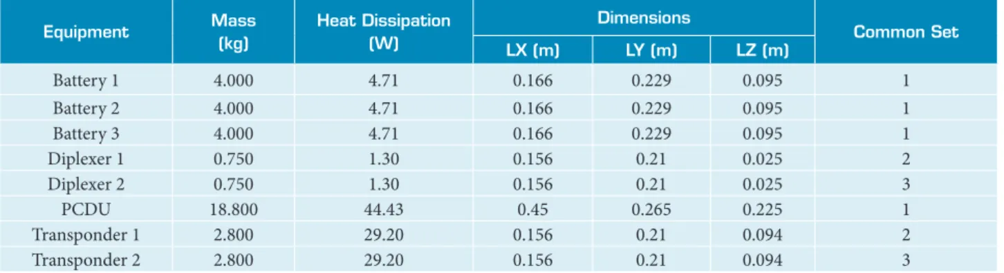
he values used for the geometric dimensions, mass, heat dissipation and common set for each equipment is shown in Table 1.
he M-GEO algorithm was used for the optimizations, starting with initial conigurations randomly generated. he number of model updates was selected as the stopping criterion. All the selected objective functions are evaluated in each model update. In both runs, a total of 500,000 model updates were evaluated, corresponding to 15,624 generations in M-GEO. he deterministic parameter τ was set to 20, the variable standard perturbation parameter σperc was set to 5%, and 5 re-initializations were used during optimizations. he stored non-dominated solutions were limited to a maximum of 100 solutions.
In the irst run, with two objective functions (f2, f3), 89 non-dominated feasible solutions were recovered at the end of this search. he obtained approximate Pareto frontier is shown in Fig. 10. he large number of non-dominated solutions makes
Table 1. Geometric, mass, power and common set data of the equipment.
Equipment Mass
(kg)
Heat Dissipation (W)
Dimensions
Common Set LX (m) LY (m) LZ (m)
Battery 1 4.000 4.71 0.166 0.229 0.095 1
Battery 2 4.000 4.71 0.166 0.229 0.095 1
Battery 3 4.000 4.71 0.166 0.229 0.095 1
Diplexer 1 0.750 1.30 0.156 0.21 0.025 2
Diplexer 2 0.750 1.30 0.156 0.21 0.025 3
PCDU 18.800 44.43 0.45 0.265 0.225 1
Transponder 1 2.800 29.20 0.156 0.21 0.094 2
Transponder 2 2.800 29.20 0.156 0.21 0.094 3
Bnd
F3 F2
Ut Ball
1.5 2 2.5 3 3.5 4
5 7 9 11 13 15 17 19 21 23
C
o
m
m
o
n
S
et
D
is
ta
n
ce
F
3
(
m
)
Heat Density - F2 (W/m2)
Figure 10. Optimization with two objective functions (F2, F3) Approximate Pareto frontier found using M-GEO.
Table 2. Optimization using two objective functions - Selected solutions on the approximate Pareto frontier.
Selection Criterion Index of solution on the approximate Pareto frontier
f2
(W/m2)
f3
(m)
Best value obtained for the thermal uniformity (f2)
objective function. F2 24 6.7826 3.7427
Best value obtained for the distance between equipment of
the same common set (f3) objective function. F3 6 20.6329 1.5931
Non-dominated solution closest to the barycenter calculated only considering the edges of the approximate
Pareto frontier.
Bnd 3 11.5459 1.9071
Non-dominated solution closest to the barycenter obtained considering all solutions on the approximate Pareto
frontier.
Ball 74 6.9032 2.3249
Non-dominated solution closest to the utopian solution. Ut 31 7.1172 1.9220
picked from the frontier. hey are presented in Table 2 and shown in Fig. 10.
In Fig. 11, colors were used to distinguish equipment of common sets: green for set 1, blue to set 2, and orange for set 3.
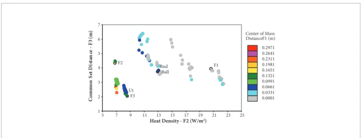
In the second run, with three objective functions (f1, f2,
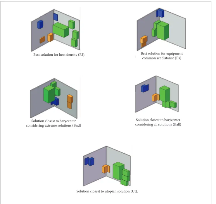
f3), 100 non-dominated feasible solutions were recovered. Figure 12 shows a plot of all these solutions. A colored scale was used to represent the f1 objective function. Table 3
presents the six selected solutions and Fig. 13 shows their layout conigurations.
he results shown on Figs. 10 and 12 shows clearly the capacity of the layout tool generate a great number of feasible non-dominated solutions for a 3D problem, starting from a completely random coniguration. he two objective functions in the irst optimization run are naturally competitive: the heat density f2 drives the layout to a spread equipment coniguration to avoid “hot” spots, while the common set distance f3 drives
Figure 11. Optimization with Two Objective Functions - Layout conigurations for selected solutions. Best solution for heat density (F2).
Solution closest to barycenter considering extreme solutions (Bnd)
Solution closest to utopian solution (Ut).
considering all solutions (Ball) Best solution for heat density (F2). Best solution for equipment
common set distance (F3)
common set distance (F3)
considering extreme solutions (Bnd)
o equipment to dense clusters in order to reduce the distances
between equipment. Plotting the results with these two functions as coordinate axis highlights this competitive behavior. While the mass center objective function may not conlict with heat density and the equipment common set ones, it drives the search towards equipment coniguration which mass center
position is close to the desired one. Examining, in Figs. 11 and 13, the solutions selected using the automatic decision making criteria, it can be seen clearly that the edge criteria generate very diferent layout solutions, due to the fact that they represent trade-of solutions that privileges one of the objective functions. On the other hand, the solutions chosen using the barycenter
F3
F1 F2
Bnd Ball
Ut
1 2 3 5
4 6 7
5 7 9 11 13 15 17 19 21 23 25
C
o
m
m
o
n
S
et
D
is
ta
n
ce
- F
3
(m
)
Heat Density - F2 (W/m2)
Center of Mass Distance F1 (m)
0.2971 0.2641 0.2311 0.1981 0.1651 0.1321 0.0991 0.0661 0.0331 0.0001
Figure 12. Optimization with Three Objective Functions - Approximate Pareto frontier found using M-GEO.
Table 3. Optimization with Three Objective Functions - Selected solutions on the approximate Pareto frontier.
Selection Criterion
Index of solution on the approximate Pareto
frontier
f1
(m)
f2
(W/m2)
f3
(m)
Best value obtained for the mass center (f1)
objective function. F1 5 0.0001 20.6003 3.9522
Best value for the thermal uniformity (f2)
objective function. F2 16 0.1981 6.7834 4.3506
Best value for the distance between equipment
of the same common set (f3) objective
function.
F3 2 0.1457 8.5488 2.0540
Non-dominated solution closest to the barycenter calculated only considering the
edges of the approximate Pareto frontier.
Bnd 57 0.0705 12.9192 3.7523
Non-dominated solution closest to the barycenter obtained considering all solutions
on the approximate Pareto frontier.
Ball 58 0.0553 13.0616 3.8427
Non-dominated solution closest to the
or utopian approach, are less dissimilar, but still provide a lot of information on alternative design solutions. Conirming what was observed previously for the two dimensional test example (De Sousa et al., 2013), it is noteworthy how the layout tool can provide potentially signiicant design gains. For example, in the present 3D application with three objective functions, a 38 % reduction on the value of objective function f3 is obtained
if solution Ut is chosen instead of solution F1. In a real design application this would mean a signiicant reduction on the cabling connecting the equipment, which can lead, for example, to cost savings and mitigation of integration problems.
he processing time spent for running each optimization was approximately 3 hours and 32 minutes, in a PC with a Core i5 CPU, 2.5 GHz of clock and 4 GB of RAM memory.
Figure 13. Optimization with Three Objective Functions - Layout conigurations for selected solutions. Best solution for center of mass (F1).
Best solution for equipment common set distance (F3)
Solution closest to barycenter considering extreme solutions (Bnd)
Solution closest to utopian solution (Ut). Solution closest to barycenter
considering all solutions (Ball)
Solution closest to utopian solution (Ut). considering all solutions (Ball)
o
CONCLUSIONS
In this paper a tool for three dimensional multidisciplinary design conception of spacecraft equipment layout was presented. It is an evolution of an early prototype with 2D capability, which main features where presented in COBEM 2013 (De Sousa et al., 2013). he tool can be used either as a research bed for testing diferent candidate methodologies and optimization algorithms to the problem, as well as an operational tool to be used by an engineering design team. he choice of using Excel
®
as the main sotware platform over which the optimization tool is built, was based on the convenience of having a readily available and broadly known sotware, which could be easily used for data input, numerical calculations, output of results and integrator of CAD or CAE sotware.he tool uses Cuco’s multiobjective methodology (Cuco, 2011; Cuco et al., 2014) as the main framework for the layout optimization, which is performed by a customized implementation of the M-GEO (Galski, 2006) algorithm. he search for the optimal solutions, the approximate Pareto set, is performed from an initial completely random layout coniguration. he user can select up to 5 diferent objective functions to guide the search. he user can also set which spacecrat panel’s faces are available for positioning a given set of equipment. Excel
®
was coupled to SolidWorks®
, which is used to calculate design parameters and as a graphical interface,where candidate layout conigurations can be visualized. Results are automatically retrieved to a dedicated Excel
®
worksheet, becoming available to be further analyzed, either graphically or using internal Excel®
features. he tool also embodies an automatic decision making procedure to select solutions on the approximate Pareto frontier, which, for a frontier with many non-dominated solutions, may help the user to decide which of them are more suitable to be further investigated. All these characteristics were exercised in a simpliied three dimensional application example, which highlighted the potential beneits such a tool can provide.he Excel
®
based spacecrat equipment layout tool presented in this paper can be considered the irst “operational” version of a tool which preliminary results were presented at COBEM 2013 (De Sousa et al., 2013). It was conceived to be continuously improved with new features, and short term goals in its development are the inclusion of new optimization algorithms and new objective functions to address additional engineering issues, as well as its application to a full real spacecrat layout problem. his would imply in a much larger design problem. For instance, for the service module of a middle size satellite of 500 kg, such as the MMP (Multi-Mission Platform) developed currently at INPE, the sotware would have to deal with around 88 design variables (for example, 22 equipment each one with four design variables). Moreover, there may be an increase in the number of constraints, depending on requirements posed on the positioning of some equipment.REFERENCES
Baier, H. and Pühlhofer, T., 2003, “Approaches for further rationalization in mechanical architecture and structural design of satellites”, In Proceedings of 54th International Astronautical Congress, Bremen, Germany.
Cuco, A.P.C., 2011, “Development of a Multiobjective methodology for layout optimization of equipment in artiicial satellites” (in Portuguese), Master dissertation, Postgraduate Course in Space Technology and Engineering, National Institute for Space Research (INPE).
Cuco, A.P.C, De Sousa, F.L. and Silva Neto, A.J., 2014, “A multi-objective methodology for spacecraft equipment layouts”, Optimization and Engineering. doi:10.1007/s11081-014-9252.
De Sousa, F.L., Muraoka, I. and Galski, R.L., 2007, “On the optimal positioning of electronic equipment in space platforms”, In Proceedings of the 19th International Congress of Mechanical Engineering, Brasilia, Brasil.
De Sousa, F.L., 2002, “Otimização extrema generalizada: um novo algoritmo estocástico para o projeto ótimo”, (INPE-9564-TDI/836), Ph.D. Thesis in Computação Aplicada, Instituto Nacional de Pesquisas Espaciais, 142p.
De Sousa, F.L., Ramos, F.M., Paglione, P. and Girardi, R.M., 2003, “New stochastic algorithm for design optimization”, AIAA Journal, Vol. 41, No. 9, pp. 1808-1818.
De Sousa, F.L. and Takahashi, W.K., 2005, “Generalized Extremal Optimization Applied to Three-Dimensional Truss Design”, Proceedings of the 18th International Congress of Mechanical Engineering (COBEM2005), CDROM, Ouro Preto, Brasil.
De Sousa, F.L., Galski, R.L., Rocco, E.M., Becceneri, J.C., Santos, W.A. and Sandri, S.A., 2013, “A toll for multidisciplinary design conception of spacecraft equipment layout”, 22nd International Congress of Mechanical Engineering (COBEM, 2013), Ribeirão Preto, SP, Brazil.
Galski, R. L., 2006, “Desenvolvimento de versões aprimoradas híbridas, paralela e multiobjetivo do método da otimização extrema generalizada e sua aplicação no projeto de sistemas espaciais”, (INPE-14795-TDI/1238), Ph.D. Thesis in Computação Aplicada, Instituto Nacional de Pesquisas Espaciais, São José dos Campos, Brazil, 279p.
Hengeveld, D.W., Braun, J.E., Eckhard, A.G. and Williams, A.D., 2011, “Optimal placement of electronic components to mininize heat lux nonuniformities”, Journal of Spacecraft and Rockets, Vol. 48, No. 4, pp. 556-563. doi: 10.2514/1.47507.
Jackson, B. and Norgard, J., 2002, “A stochastic optimization for determining spacecraft avionics box placement”, IEEE Aerospace Conference, Vol. 5, pp. 2373-2382.
Ferebee Jr., M.J. and Powers, R.B., 1987 “Optimization of payload mass placement in a dual keel space station”, NASA Technical Memorandum 89051, March.
Ferebee Jr. M.J. and Allen C.L., 1991. “Optimization of payload placement on arbitrary spacecraft”, Journal of Spacecraft and Rockets, Vol. 28, No. 5, pp. 612-614. doi: 10.2514/3.26288.
Mainenti-Lopes, I., De Sousa, F.L. and Souza, L.C.G., 2008, “The Generalized Extremal Optimization With Real Codiication”. Proceedings of International Conference on Engineering Optimization – EngOpt2008, Rio de Janeiro, pp. 01-05.
Mainenti-Lopes, I, Souza, L.C.G. and De Sousa, F.L., 2012, “Design of a nonlinear controller for a rigid-lexible satellite using multi-objective Generalized Extremal Optimization with real codiication”, Shock and Vibration, Vol. 19, No. 5, pp. 947-956. doi: 10.3233/ SAV-2012-0702.
Mainenti-Lopes, I., 2013, “A Multiobjective Approach to the Optimization of Solar Sail Trajectories” (In Portuguese), Ph.D. Thesis, Pós-graduação em Engenharia e Tecnologia Espaciais, área Mecânica Espacial e Controle, INPE.
Pühlhofer, T., Langer, H., Baier, H. and Huber, M., 2004, “Multicriteria and discrete coniguration and design optimization with applications for satellites”, In Proceedings of 10th AIAA/ISSMO Multidisciplinary Analysis and Optimization Conference, Albany.
Rocco, E.M., Souza, M.L.O. and Prado, A.F.B.A., 2003, “Multi-Objective Optimization Applied to Satellite Constellations I: Formulation of the Smallest Loss Criterion”, Proceedings of the 54st International Astronautical Congress (IAC’03), Bremen, Germany.
Rocco, E.M., Souza, M.L.O. and Prado, A.F.B.A., 2013, “Station Keeping of Costellations Using Multiobjective Strategies”, Mathematical Problems in Engineering, Hindawi Publishing Corporation, Vol. 2013, pp. 15. doi:10.1155/2013/476451.
Sun, Z-G and Teng, H-F., 2003, “Optimal layout design of a satellite module”, Engineering Optimization, Vol. 35, No. 5, pp. 513-529.
Teng, H-F, Sun, S-L, Liu, D-Q and Li, Y-Z., 2001, “Layout optimization for the objects located within a rotating vessel – a three-dimensional packing problem with behavioral constraints”, Computers and Operations Research, Vol. 28, pp. 521-535.
Teng, H-F., Chen, Y., Zeng, W., Shi, Y-J. and Hu, Q-H., 2010, “A Dual-system variable grain cooperative coevolutionary algorithm: satellite-module layout design”, IEEE Transactions on Evolutionary Computation, Vol. 14, No. 3, pp. 438-455.
Vanderplaats, G., 2007, “Multidiscipline Design Optimization”, Vanderplaats Research and Development Inc. ISBN 0-944956-04-1.
Venditti, F.C.F., Rocco, E.M., Prado, A.F.B.A. and Suhkanov, A., 2010, “Gravity-assisted maneuvers applied in the multi-objective optimization of interplanetary trajectories”, Acta Astronautica, Elsevier Ltd., Vol. 67, No. 9–10, pp. 1255–1271. doi.:10.1016/j. actaastro.2010.06.022.