Braz. J. Chem. Eng. vol.21 número4

(1)

ISSN 0104-6632 Printed in Brazil

Vol. 21, No. 04, pp. 557 - 568, October - December 2004

Brazilian Journal

of Chemical

Engineering

A CFD MODEL FOR POLLUTANT

DISPERSION IN RIVERS

K. Modenesi

1

, L. T. Furlan

2

, E. Tomaz

1

, R. Guirardello

1

and J. R. Núnez

1*

1

Faculdade de Engenharia Química, Departamento de Processos Químicos,

UNICAMP - Universidade Estadual de Campinas, Cidade Universitária Zeferino Vaz, 13083-970 Fone +(55) (19) 3788-3967, Campinas - SP - Brazil

2

REPLAN/PETROBRAS, Rodovia SP-332, Km 132, Paulínia - SP, Brazil, E-mail: kelerson@feq.unicamp.br, E-mail: furlan@petrobras.com.br

E-mail: etomaz@feq.unicamp.br, E-mail: guira@feq.unicamp.br E-mail: nunhez@feq.unicamp.br

(Received: August 28, 2003 ; Accepted: June 4, 2004)

Abstract - Studies have shown that humankind will experience a water shortage in the coming decades. It is therefore paramount to develop new techniques and models with a view to minimizing the impact of pollution. It is important to predict the environmental impact of new emissions in rivers, especially during periods of drought. Computational fluid dynamics (CFD) has proved to be an invaluable tool to develop models able to analyze in detail particle dispersion in rivers. However, since these models generate grids with thousands (even millions) of points to evaluate velocities and concentrations, they still require powerful machines. In this context, this work contributes by presenting a new three-dimensional model based on CFD techniques specifically developed to be fast, providing a significant improvement in performance. It is able to generate predictions in a couple of hours for a one-thousand-meter long section of river using Pentium IV computers. Commercial CFD packages would require weeks to solve the same problem. Another innovation inb this work is that a half channel with a constant elliptical cross section represents the river, so the Navier Stokes equations were derived for the elliptical system. Experimental data were obtained from REPLAN (PETROBRAS refining unit) on the Atibaia River in São Paulo, Brazil. The results show good agreement with experimental data.

Keywords:Computational fluid dynamics ,pollutant dispersion in rivers.

INTRODUCTION

During many decades the growth of urban centers and industries occurred without any controls. The consequences of this lack of organization are felt everywhere. The effects of human activities resulting in the pollution of water, soil and air have been widely studied and discussed at many research centers. People are taking notice of the risks involved in the misusage of natural resources. Specifically, the possibility of shortages of fresh water resources in the near future has increased, and in some places populations already suffer this effect. Some regions of the world experience daily rationing

of drinking water. These facts have increased the interest of industries and environmental agencies in the development of research activities and programs aiming to reduce effluent emissions and to predict the environmental impact of new emissions as well as to treat already polluted bodies of water.

(2)

and Wu et. al. (2000)).

Many researchers are also interested to determine which turbulent models are appropriate to the closure of the turbulence model ((Lane et. al, 1998). and Ye and McCorquodale (1998)).

The modeling of particle dispersion has also proved to be a theme of interest for many. Nokes and Hughes (1994) proposed a turbulent three-dimensional model to study turbulent dispersion in open channels containing arbitrary, but constant, dimensions. In this method, a semi-analytic technique was applied to study the permanent discharge of a non-degenerative effluent in a channel of known velocity and diffusivity distributions. The model assumed that no secondary fluxes were present; reflecting a limitation of the original mathematical model. Shiono and Knight (1991) and Tominaga and Nezu (1991) showed that even channels with simple shapes have secondary flows. Using a k-ε model, Naot and Rodi (1982) showed that secondary flows also appear near walls in channels with regular cross sections.

The main contribution of the present work is that it proposes a three-dimensional model capable of predicting the dispersion of effluents in open channels using a very fast in-house code, an unusual feature for CFD models. Due to this, it is possible to predict the dispersion of substances in sections of rivers kilometers long, so the end product of this research has applications as a predictive tool to support and guide management decisions of an industrial nature.

Some of the results obtained through use of the software are presented in this work. This software is based on the three-dimensional model of the dispersion of an inert effluent using CFD techniques. Velocity and concentration profiles for the substance are obtained through the numerical solution of the conservation of mass and momentum equations. Results of a case study in which experimental data were used for model validation are shown. As already mentioned, a distinctive feature of the software is its speed. For a one-thousand-meter long section of river, only about one hour of CPU time on a Pentium IV computer was required to generate the results. A commercial package would have taken several days to run a similar problem.

MODEL FORMULATION

The discrete form of the equations of continuity, motion and mass conservation generated by the mathematical model were solved to determine the

velocity and concentration profiles for the substance being discharged into the river. The full equations, in their free-coordinate form, are given by

( )

div 0

t

∂ρ + ρ =

∂ v

r

(1)

D

grad p div

Dt

ρ v= ρ −g + t

r

r r

(2)

2 A

G A A

DC

K C R

Dt = ∇ + (3)

The above equations are simplified, taking into consideration the following hypotheses assumed for the model:

§Flow is laminar;

§Flow is fully developed along the z direction; §The velocity distribution is independent of the downstream coordinate, z;

§There is no secondary flow in the channel, so the downstream velocity (z direction) is the only nonzero velocity component;

§There are no interactions between the river bed and the water.

§The dispersing plume is long and thin, so the

diffusion term in the z direction is negligible in comparison with the convective term in the same direction;

§Newtonian fluid;

§Physical properties, including global dispersion and volatility coefficients, are constant;

§No chemical reaction.

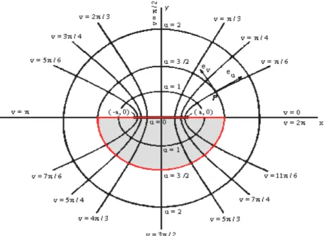
The shape of the river was represented by a half-cylinder channel with a constant elliptical cross section, so it is possible to set both the depth and the width of the river. The adoption of this shape is an original aspect of this study. The best coordinate system to represent this shape is the elliptic cylindrical one. Figure 1 illustrates this coordinate system (Spiegel, 1972).

Taking into consideration the hypotheses, the equations of the model, written in an elliptic cylindrical coordinate system, are shown below:

z

v 0 z

∂ =

∂ (4)

( )

₍

₎

2 z 2 z

2 2

2 2 2

v v

0 g sin

u v

a senh u sen v

_∂ _∂ 

µ

= ρ θ + _ + _

∂ ∂

(3)

(

)

2 2

A A A

z G ₂ ₂ ₂ ₂ ₂

C 1 C C

v K

z a senh u sen v u v

 _ _

∂ ₌ _ _∂ ₊∂ __

 

 

∂ _ +  ∂ ∂ _ (6)

The boundary conditions for the model are presented as follows:

§ Velocity is equal to zero on the bed of the river

à vz =0;

§ The shear stress is set to zero on the water surface

à z

i

v 0 n

∂ =

∂ ;

§ A concentration distribution is specified as an inlet condition _àC_A

(

u, v, 0

)

=C_A0

(

u, v

)

;

§ Flux of material across the bed of the river is set to

zero à A

i

C 0 n

∂ ₌

∂ ;

§Flux of material across the water surface is not

zero _à A _V _A

i

C

K C

n

∂ ₌ _⋅

∂ ;

Where n_i is the ith component of the outward boundary unit normal to the boundary, and

KV is the volatilization coefficient of the dispersing

contaminant.

Ammonia compounds, which are studied in this work, are volatile. This characteristic is represented in the model through the use of a volatilization coefficient, so that the loss of mass through evaporation at the river surface can be considered.

Figure 1: Elliptic cylindrical coordinate system in an x-y plane.

NUMERICAL PROCEDURE

Basically, the solution approximation for the model is carried out in two steps. First, the velocity profile is calculated. Then, using these results, the concentration distributions of the contaminant in the river are obtained.

The velocity profiles are calculated through solution of equation 5 using a fourth-order finite differences method. The first term on the right side of equation 5 was determined iteractively using the volumetric flow rate of the river and of the effluent and the equation of mass conservation.

Using the calculated velocity profile, it is possible to determine the distribution of concentrations in the

river by solving equation 6. A fourth-order Runge-Kutta method and a second-order finite differences scheme were used. The numerical discrete equations obtained from the model equations for the elliptical geometry are listed below:

Axial Velocity

(4)

i = 1 i = 2 i = 3 i = 4 i = N-2 i = N-1 i = N i = N+1

j = 1 j = 2 j = 3 j = 4 j = M-2 j = M-1 j = M j = M+1

v = π u = up

u = 0

v = 2 π

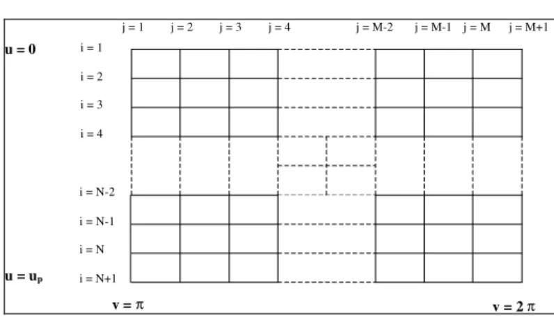
Figure 2: Mesh used for the discretization

Equation 7 is valid for the whole domain, except at the boundaries, where the boundary conditions are applied. The numerical scheme used is the fourth order finite differences method. The general term (where the boundary conditions do not apply) the numerical equations are given by:

i j

2 2

z z

1 i i

2 2

u v

i j

v v

K F(u , v ) ;

u v

u (i 1) u ; v ( j 1) v

_∂ _∂ 

 ₊ ₌ _⋅

 _∂ _∂ 

 

 

= − ∆ = π + − ∆ (7)

where

L

H

g

K

₁

µ

⋅

ρ

=

and

(8)

(

senh

u

sen

v

)

a

)

v

,

u

(

F

=

−

2 2

+

2

i = 3, 4, ..., N-1

j = 3, 4, ..., M-1

(

)

i 2,j i 1, j i,j i 1, j i 2,j i,j 2 i,j 1 i,j i,j 1 i,j 2

2 2

1 i j

Vz 16 Vz 30 Vz 16 Vz Vz Vz 16 Vz 30 Vz 16 Vz Vz

12 u 12 v

K F u , v

− − + + − − + + − + ⋅ − ⋅ + ⋅ − − + ⋅ − ⋅ + ⋅ − + = ∆ ∆ = ⋅ (9)

The linear system has _

(

N 1+ ⋅

) (

M 1+ 

)

_ equations, referring to the velocities to be determine plus the K1

constant1. which is determined using the mass flowrate.

ConcentrationProfile

From the boundary conditions the equations for the concentration are:

i = 1 j = 1, 2, ..., M+1

3 C

C

4 C

A 2,j A 3,j

j , 1 A

−

⋅

=

(10)

i = N+1 j = 1, 2, ..., M+1

3 C

C

4 C

A N,j A N 1,j

j , 1 N A − +

−

⋅

=

(11)

i = 2, ... , N j = 1

3 C

C

4 C

A i,2 A i,3

1 , i A

−

⋅

=

(12)

i = 2, ... , N

3 C

C

4 C

A i,M A i,M 1

1 M , i A − +

−

⋅

=

(13)

i = 2, ... , N j = 2, ..., M

( )

[

]

[

( )

]

{

senh i 1 u sen i 1 v

}

a v C C 2 C u C C 2 C v K dz C d 2 2 2 2 1 j , i A j , i A 1 j , i A 2 j , 1 i A j , i A j , 1 i A j , i z G j , i A ∆ − + π + ∆ −         ∆ + ⋅ − + ∆ + ⋅ − = − + −

(5)

Equations 10-14 are solved using a Runge-Kutta fourth order scheme.

RESULTS

In order to test the results, the velocity distribution for the elliptical system was compared with the results for the cylindrical system, where an analytical solution for the laminar case is known. In order to compare results of the two-coordinate systems, the simulations were carried out according to Table1. I should be noticed that the height in a cylindrical system is readily obtained as being half of

the diameter (width of the river). When comparing to the elliptical system, this condition cannot be achieved because the two focal points of the elliptical system cannot coincide. In this case, two limiting cases approaching this condition were tested, that is h=4.999 and h=5.001.

Figure 2 shows the velocity results at the free surface and on a plane at the centerline of the river. The results are identical, as expected.

A software has been developed based on the mathematical model. In order to verify the applicability of the model, the results of a case study on a river having the dimensions and flow characteristics according to Table 2 are shown.

Table 1: Comparison for the elliptical and cylindrical systems.

W [m] h [m]

Case 1 Elliptical 10.0 4.999

Case 2 Cylindrical 10.0 5.000

Case 3 Elliptical 10.0 5.001

Velocity distribution at the free surface of the river

-6 -4 -2 0 2 4 6

0 0.1 0.2 0.3 0.4 0.5 0.6

Velocity [m/s]

Width [m]

Case 1 Case 2 Case 3

Velocity distribution on a plane at the centerline of the river

-2 -1 0

0 0.1 0.2 0.3 0.4 0.5 0.6

Velocity [m/s]

Depth [m]

Case 1 Case 2 Case 3

(a) (b)

Figure 3:Velocity results at the free surface (a) and a centerline (b) of the river.

Table 2: Data for a case example.

h [m] 3.00

W [m] 10.00

L [m] 1,000.00

Qr [m 3

/s] 10.00

Qe [m3/s] 0.10

KG [m2/s] 0.02

KV [1/m] 0

CA0 [mg/l] 0.50

(6)

KV is a coefficient accounting for any

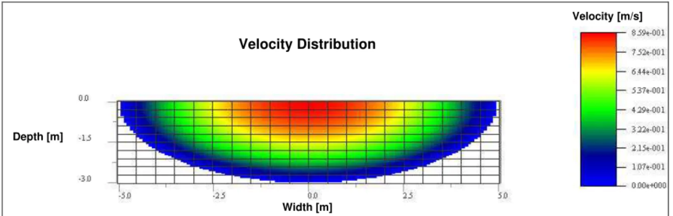
volatilization at the river surface. The null value means that the polluting substance does not volatize at the surface. The global dispersion coefficient is within the range of values experimentally determined by Fischer (1967). The results presented in Figure 4 have been obtained for the velocity contour plot.

The model indicates that the maximum velocity is at the centerline on the surface of the river (see Figure 4). Some experimental publications have shown that the maximum velocity actually occurs just below the free surface of the river. This happens because, in practice, there are tensions at the free surface that were not taken into consideration by this model (e.g. those caused by wind). If need be, these can be considered in future refinements of the model.

Figure 5 shows the cross-sectional concentration profile located at 0, 50, 100, 150, 250, 350 and 485 meters. The red color indicates a high effluent concentration. The model shows the effluent being dispersed until it is diluted at a distance LD = 485m,

where the concentration at any point of the session is (0.554 mg/l ± 0.5%). In this work this distance is called the dilution distance.

The following plot (Figure 6) shows the effluent being dispersed at the free surface of the river. It should be observed that the range of variation in concentration in Figure 6 is from 0.5 to 5 mg/l. This choice allows for a better visualization of the results. Otherwise, the variation would be visualized only very close to the emission of effluent. As already shown in Figure 5, concentration does not vary considerably after 485 meters.

Velocity Distribution

Width [m] Depth [m]

Velocity [m/s]

Figure 4: Contour plot of velocity for the case study.

Concentrations at z = 0.0 m

Concentration [mg/ l]

(7)

(b) - cross-sectional concentration profile 50m away from the discharge point

(c) - cross-sectional concentration profile 100m away from the discharge point

(8)

(e) - cross-sectional concentration profile 250m away from the discharge point

Depth [m]

Width [m]

(f) - cross-sectional concentration profile 350m away from the discharge point

Concentration at z = 485.0 m

Depth [m]

Width [m]

(g) - cross-sectional concentration profile 485m away from the discharge point

(9)

Concentration distribution at the free surface of the river

Width [m]

Length [m]

Figure 6: Contour plot of concentration at the river surface.

Comparison with Experimental Data

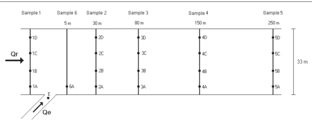
The experimental data used in this work were obtained from the Atibaia River in the state of São Paulo in Brazil, where effluent is discharged from several industries, including REPLAN, a major unit of the PETROBRAS Refining Industry. Figure 7 shows the distances from the river discharge point where the experimental data were collected. The sampling distances (3m, 11m, 22m and 30m) are measured across the Atibaia river.

The dimensions of the river were measured when

the data were collected. The volumetric flow rate of the effluent was given by the refinery. These data are shown in Table 3.

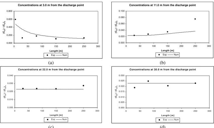
Figure 8 compares the total chloride concentrations given by the model and by the experimental data. The results show reasonable agreement.

Figure 9 shows the dimensionless concentration of ammonium along the river. In this case, the loss of ammonia at the free surface of the river was accounted for by the model. The results follow the trend of the experimental data.

Figure 7: Schematic representation of the sample points.

Table 3: Data on the Atibaia River and REPLAN effluent.

W [m] 33.0

h [m] 3.0

L [m] 250.0

Qr [m 3

/s] 20.0

(10)

Concentrations at 3.0 m from the discharge point 0.000 0.200 0.400 0.600 0.800

0 50 100 150 200 250 300

Length [m]

(C

Cl

) / (C

Cl

)e

Exp Num

Concentrations at 11.0 m from the discharge point

0.000 0.020 0.040 0.060 0.080 0.100

0 50 100 150 200 250 300

Length [m]

(C

Cl

) / (C

Cl

)e

Exp Num

(a) (b)

0.000 0.010 0.020 0.030 0.040

0 50 100 150 200 250 300

L e n g t h [ m ]

(C

Cl

) / (C

Cl

)e

Exp Num

0.000 0.005 0.010 0.015 0.020 0.025 0.030

0 50 100 150 200 250 300

L e n g t h [ m ]

(C

Cl

) / (C

Cl

)e

Exp Num

(c) (d)

Figure 8: Dimensionless concentration of chloride at the free surface of the river for a segment 250 m from the effluent discharge point. The points were located at (a) 3m (b) 11 m

(c) 22 m and (d) 30 m from the river discharge point.

Concentrations 3.0 m from the discharge point

0.000 0.200 0.400 0.600 0.800

0 50 100 150 200 250 300

Length [m]

Dimensionless

concentration

Exp Num

0.000 0.050 0.100 0.150

0 50 100 150 200 250 300

Length [m]

Am

Dimensionless concentration

Exp Num

(a) (b)

0.000 0.020 0.040 0.060 0.080 0.100

0 50 100 150 200 250 300

Length [m]

Dimensionless

concentration

Exp Num

0.000 0.020 0.040 0.060 0.080 0.100

0 50 100 150 200 250 300

Length [m]

Dimensionles

concentration

Exp Num

(c) (d)

Figure 9: Variation in dimensionless concentration of ammonium at the free surface of the river for a segment 250 m from the effluent discharge point. The points were located at:

(11)

In this case, the dilution distance for the chlorides is 6920 meters. It is more difficult to establish the dilution distance for the ammonium, since the model takes into account its loss at the free surface of the river. Without considering the loss of ammonium, the dilution concentration is 0.0872. Since ammonium is lost at the free surface, after 1280 meters it is observed that no point in the river has a concentration above this value. However, there are significant differences in concentration in any cross section near that distance from the discharge point. After 5000 meters, the concentration values range from 0.048636 to 0.061574 and the average concentration for the section is 0.059158. It can be said that the concentration is very low, even though it is not homogeneously dispersed. For substances being lost at the surface, probably the best way to analyze particle dispersion is to observe after which river length no point in the cross-sectional area is above a predetermined concentration value.

A remarkable feature of this new CFD model is that it is very fast. The first case study took only 1 hour and 20 minutes to converge. This is not common in CFD codes at the time of writing this paper. This study would require many days or even weeks to solve using commercial packages.

CONCLUSIONS

The results shown in this paper indicate that this new CFD model is capable of giving detailed information on the dispersion of inert soluble particles in a river, despite the simplifications considered. The comparison between experimental data and model results indicates that the model is suitable for predicting particle dispersion. Another interesting feature of the model is that it takes into account the loss of volatized substances, when required. The computational time for the three-dimensional simulations did not exceed two hours for the first case study. The model is very fast, making it a powerful tool for risk assessment.

NOMECLATURE

CA Component A concentration in the river

CA0 Component A concentration in the river

before effluent discharge

CAe Component A concentration in the

effluent

g Acceleration due to gravity

gr

Gravitational acceleration vector

h Depth of the flow

KG Global dispersion coefficient

KV Volatility coefficient

L Length of the river segment

P Pressure

LD Dilution distance

Qe Volumetric flow rate of the effluent

Qr Volumetric flow rate of the river

RA Reaction term

t Time

u Elliptic cylindrical coordinate

v Elliptic cylindrical coordinate

v

r

Velocity vector

Vz Axial velocity component

W Width of the river segment

z Axial coordinate

t

r

Shear stress

µ Viscosity

ρ Fluid density

REFERENCES

Bradbrook, K.F.; Lane, S.N. and Richards, K.S., Numerical Simulation of Three-dimensional Time-Averaged Flow Structure at River Channel Confluences. Water Resour. Res. 36 (9), 2731-2746, 2000

Fischer, H.B., The Mechanics of Dispersion in Natural Streams, J. Hydr. Div., 93 (6), 187-216, 1967.

Lane, S.N. and Bates, P.D. Introduction in: Bates, P.D.; Lane, S.N. (Eds), High Resolution Flow Modeling in Hydrology and Geomorphology. Wiley, Chichester, pp1-12, 2000.

Lane, S.N.; Bradbrook, K.F.; Richards, K.S.; Biron, P.A. and Roy, A.G. The Application of Computational Fluid Dynamics to Natural River Channels: Three-Dimensional Versus Two Dimensional Approaches, Geomorphology, 29, 1-21 Lin Ma;, Ashworth, P.J.; Best, J.L.; Elliott, L.;

Ingham, D.B. and Whitecombe, L. J. Computational Fluid Dynamics and the

Physical Modeling of an Upland Urban River, Geomorphology, 44, 375-391, 2002

Naot, D. and Rodi, W., Numerical Simulation of Secondary Currents in a Channel Flow, J. Hydr. Div., 108 (8), 948-968, 1982.

(12)

Shiono, K. and Knight, D.W., Turbulent Open-channel Flows with Variable Depth Across the Channel, J. Fluid Mech., 222, 617-646, 1991. Spiegel, M.R., Análise Vetorial – com Introdução

à Análise Tensorial, McGrawHill do Brasil, 1972.

Tominaga, A. and Nezu, I., Turbulent Structure in

Compound Open-channel Flows, Journal of Hydraulic Engineering, vol. 117, No 1, January, 1991.