ISSN 0104-6632 Printed in Brazil
www.abeq.org.br/bjche
Vol. 24, No. 01, pp. 151 - 162, January - March, 2007
Brazilian Journal
of Chemical
Engineering
THE PERFORMANCE OF SIMULATED
ANNEALING IN PARAMETER ESTIMATION FOR
VAPOR-LIQUID EQUILIBRIUM MODELING
A. Bonilla-Petriciolet
1*, U. I. Bravo-Sánchez
1, F. Castillo-Borja
1,
J. G. Zapiain-Salinas
1and J. J. Soto-Bernal
21
Departamento de Ingeniería Química, Instituto Tecnológico de Aguascalientes, Phone and Fax: (52) 449 910-5002 ext. 127, CP: 20256, Aguascalientes, Aguascalientes, México.
Email: [email protected] 2
Departamento de Sistemas y Computación Instituto Tecnológico de Aguascalientes, CP: 20256, Aguascalientes, Aguascalientes, México.
(Received: May 30, 2005 ; Accepted: December 4, 2006)
Abstract - In this paper we report the application and evaluation of the simulated annealing (SA) optimization method in parameter estimation for vapor-liquid equilibrium (VLE) modeling. We tested this optimization method using the classical least squares and error-in-variable approaches. The reliability and efficiency of the data-fitting procedure are also considered using different values for algorithm parameters of the SA method. Our results indicate that this method, when properly implemented, is a robust procedure for nonlinear parameter estimation in thermodynamic models. However, in difficult problems it still can converge to local optimums of the objective function.
Keywords: Vapor-liquid equilibrium; Simulated annealing; Nonlinear parameter estimation; Error-in-variable
method; Global optimization.
INTRODUCTION
In many important areas of chemical, biochemical and petroleum engineering, mathematical models form the basis for the design, optimization and control of process systems (Esposito and Floudas, 1998; Englezos and Kalogerakis, 2001). Parameter estimation is a common problem in many engineering applications and is one of the steps involved in the formulation and validation of a mathematical model that describes a process of interest. Specifically, it refers to the process of obtaining values of the parameters by matching the model-based calculated values with the set of measurements (Englezos and Kalogerakis, 2001). If we use linear model equations, the problem is called linear estimation, while nonlinear estimation refers
to the more general problem where the model equations are nonlinear functions of the parameters. As indicated by Esposito and Floudas (1998), the use of nonlinear models introduces an added level of complexity into the numerical estimation of model parameters.
characteristics, we can solve a constrained or unconstrained optimization problem, which in general is nonlinear and potentially nonconvex.
Several local and global optimization methods have been used for parameter estimation in both linear and nonlinear models (Bard, 1974; Britt and Luecke, 1973; Fabries and Renon, 1975; Gmehling et al., 1977-1990; Anderson et al., 1978; Valko and Vajda, 1987; Tjoa and Biegler, 1992; Vamos and Hass, 1994; Esposito and Floudas, 1998; Gau et al., 2000; Gau and Stadtherr, 2002). Local optimization methods are not reliable for finding the global minimum of the problem; however, these methods are the most widely used. In the other hand, some applications of global optimization methods in parameter estimation have been reported by Esposito and Floudas (1998), Kleiber and Axmann (1998), Park and Froment (1998), Gau et al. (2000), Costa et al. (2000), Gau and Stadtherr (2002) and Dominguez et al. (2002).
An attractive alternative for the reliable solution of nonlinear parameter estimation is the use of stochastic optimization methods such as simulated annealing (SA) or genetic algorithm (GA). Even though these methods provide no formal guarantee for global optimization, they are reliable strategies and offer a reasonable computational effort in the optimization of multivariable functions (Michalewicz and Fogel, 1999). In fact, some papers have reported the application of SA and GA in parameter estimation using chemical engineering models (Kleiber and Axmann, 1998; Park and Froment, 1998; Costa et al., 2000).
In the context of thermodynamics, parameter estimation may also encounter computational difficulties due to the possibility of several local optimums in the objective function used as optimization criterion. As indicated by Dominguez et al. (2002), failing to identify the global optimum in parameter estimation may cause errors and uncertainties in equipment design and erroneous conclusions about model performance. In view of this, it is important to test different optimization methods to identify a reliable and efficient technique for this purpose.
In this paper, we report the application and evaluation of the SA method in parameter estimation for vapor-liquid equilibrium (VLE) modeling. We have tested the numerical performance of SA using the classical least squares and maximum likelihood approaches. Reliability and efficiency in the data-fitting procedure are also considered using different values for the algorithm parameters of the SA method.
METHODOLOGY
Problem Formulation
In accordance with Gau et al. (2000), consider that a set of observations yij of i 1,..., m= dependent
response variables from j 1,..., ndat= experiments is available, where the responses will be adjusted to an
explicit model yij fi x ,j
→ →
= θ
with independent
variables xj
(
x ,..., x1j pj)
T→
= and parameters
(
)
T1,..., q
→
θ = θ θ . Measurement errors in xj
→
can
either be treated or neglected, and depending on the choice, we can have a least squares or maximum likelihood formulation. Different objective functions can be used to obtain the parameter values that provide the best fit. For the case of the classical least squares (LS) criterion, we use the following objective function
2
j ij i ndat m
obj
ij j 1 i 1
y f x ,
F
y
→ → = =
− θ
=
∑∑
(1)This function is optimized with respect to the model
parameters →θ = θ
(
1,...,θq)
T and Gmehling et al. (1977-1990), Gau et al. (2000) and Dominguez et al. (2002) have used this formulation in data fitting for VLE modeling.If we assume that there are measurement errors in the state variables zij for the experiments in the
system to be modeled, the error-in-variable (EIV) formulation has the form
(
t)
2ndat nest
ij ij
obj 2
i j 1 i 1
z z
F
= = − =
σ
∑∑
(2)subject to
t ij
g z , 0 i 1,..., nest j 1,..., ndat → →
θ = = =
(3)
the number of state variables, ztij represents the unknown “true” values of state variables for each
measurement and σi represents the standard
deviation associated with the measurement of state variable i. The optimization variables of this problem
are the set of ztij and the model parameters
(
)
T1, ..., q
→
θ = θ θ . In this case, there is a substantial increase in the dimensionality of the optimization problem, which depends on the number of experiments. Esposito and Floudas (1998) and Gau and Stadtherr (2002) have applied their deterministic optimization approaches to solving Eqs. [2] and [3] with different chemical engineering models including vapor-liquid equilibrium equations.
The last functions can be minimized either as a constrained or as an unconstrained optimization problem. In all our examples, we will consider only the unconstrained formulation. We have studied the numerical performance of the SA method in the global minimization of these functions using vapor-liquid equilibrium models. In the next section, we describe the algorithm used for the SA method.
Simulated Annealing (SA)
Simulated annealing is a stochastic optimization technique inspired by the thermodynamic process of cooling of molten metals to attain the lowest free energy state (Kirkpatrick et al., 1983). Starting with an initial solution and armed with adequate perturbation and evaluation functions, the algorithm performs a stochastic partial search of the state space. In minimization problems, uphill moves are occasionally accepted with a probability controlled by a parameter called annealing temperature, TSA.
The probability of acceptance of uphill moves decreases as TSA decreases. At high temperatures,
the search is almost random, while at low temperatures the search becomes almost greedy. At zero temperature, the search becomes totally greedy, i.e., only good moves are accepted (Kirkpatrick et al., 1983). The core of the algorithm is the Metropolis procedure, which simulates the annealing process at a given TSA (Metropolis et al., 1953). The Metropolis criterion is used to accept or reject the
uphill moves. Several algorithms have been proposed for the SA method. We have used the algorithm proposed by Corana et al. (1987) because previous papers have reported its reliability and efficiency in thermodynamic calculations (Henderson et al., 2001; Rangaiah, 2001).
In the algorithm proposed by Corana et al. (1987), a trial point is randomly chosen within the step length VM (a vector of length n variables) of a starting point. The function is evaluated at this trial point and its value is compared to its value at the initial point, where the Metropolis criterion is used to accept or reject the trial point. If the trial point is accepted, the algorithm moves on from that point. If it is rejected, another point is chosen instead for a trial evaluation. Each element of VM is periodically adjusted so that half of all function evaluations in that direction are accepted. A fall inTSA, after NT iterations, is imposed upon the system with the RT variable by
SA j 1 SA j
T + =RT×T (4)
where j is the iteration counter and RT is the temperature reduction factor. For our examples, we have defined this parameter equal to 0.85 which is the value suggested by Goffe et al. (1994). Thus, as TSA declines, downhill moves are less likely to be accepted and the percentage of rejections rises. Given the scheme for the selection of VM, VM falls. Thus, as TSA declines, VM falls and SA focuses upon the most promising area for optimization. A full description of this algorithm is found in Corana et al. (1987) and we have used the subroutine developed by Goffe et al. (1994). Figure 1 shows a flow diagram of this optimization method. The choice of cooling schedule is a crucial aspect in the implementation of SA because it affects the numerical performance of the optimization procedure. Considering this fact, we have tested the effect of parameters TSA and NT on
Figure 1: Flow diagram of SA optimization algorithm (Corana et al., 1987)
RESULTS AND DISCUSSION
We test the SA method in the data-fitting procedure using several experimental VLE data and different thermodynamic models. All systems used in this paper have an objective function with multiple optimums and they have been applied for testing global deterministic optimization methods (Esposito and Floudas, 1998; Gau et al., 2000; Gau and Stadtherr, 2002). The reliability and efficiency of SA is evaluated based on the following criteria: a) success rate in finding the global minimum SR and b) average number of objective function evaluations
during the optimization procedure NFEV. All examples are solved 100 times (each time with a different random initial value and random number seed) and the results obtained are divided into four groups (each group with 25 calculations). For each group of results, SR and NFEV are calculated and a variance analysis is performed to establish the effect of parameters TSA and NT on the reliability of the
data-fitting procedure. We consider the statistical effect of these parameters significant if the value of the p-level obtained from the statistical analysis is lower than 0.05. In all our examples, we have used a tolerance of 1.0E-09 for the convergence of the SA
Initialize parameters
NT, RT, TSA
Perform a cycle of random moves, each in a coordinate direction. Accept or reject each point according to the Metropolis criterion. Record the optimum point reached so far.
No. cycles ≥
Ns
Adjust step vector VM
Reset No. cycles to 0
No. step adjustments ≥
Reduce temperature. Reset No. Adjustments to 0. Set current point to the optimum.
Stopping criterion
End
No
No Yes
Yes
No
algorithm. The experimental data are taken from DECHEMA and Reid et al. (1987). In all examples, we have assumed gas ideal behavior and the vapor pressures of pure components are calculated using the Antoine equation. For problems 1 – 4, we use the constants reported in DECHEMA for the Antoine equation.
Problem 1. Tert Butanol-1 Butanol
Our first example is the VLE for the binary system tert butanol-1 butanol. This system was studied by Gau et al. (2000) using an interval analysis approach and classical least square formulation. We use three sets of experimental data under different isobaric conditions. The Wilson equation is used to calculate the liquid-phase activity coefficients, which are defined by
1 1 12 2
12 21
2
1 12 2 21 1 2
ln ln(x x )
x
x x x x
γ = − + Λ +
Λ Λ
+ −
+ Λ Λ +
(5)
2 2 21 1
12 21
1
1 12 2 21 1 2
ln ln(x x )
x
x x x x
γ = − + Λ −
Λ Λ
− −
+ Λ Λ +
(6)
The binary parameters Λ12 and Λ21are given by
2 1
12 1 v
exp
v RT
θ
Λ = −
(7)
1 2
21 2 v
exp
v RT
θ
Λ = −
(8)
where v1 and v2 are the pure component liquid
molar volumes, T is the system temperature and θ1
and θ2 are the energy parameters. Assuming an ideal vapor phase, the experimental values for the
activity coefficients γexpi are calculated using the next equation
exp exp exp i i exp 0
i i
y P
i 1,..., c
x P
γ = = (9)
where Pi0 is the vapor pressure of pure component i at the system temperature T and c is the number of components. The vapor pressure is calculated using
0 1
10 i 1 1
b
log P a
c T
= −
+ (10)
where T is in °C andPi0, in mmHg. In accordance with Gmehling (1977-1990) and Gau et al. (2000), we use a relative least squares formulation to fit the data
2 exp calc ndat c
ij ij
obj exp
j 1 i 1 ij F
= =
γ − γ
=
γ
∑∑
(11)We optimize this function with respect to the Wilson model parameters inside the intervals
1 ( 8500, 320000)
θ ∈ − and θ ∈ −2 ( 8500, 320000).
The initial values for each calculation are randomly generated within these intervals. The performance of SA is tested using the next arbitrary values for its parameters: TSA(10, 100, 1000) and NT (10, 20). The results obtained by other thermodynamic calculations suggest that our proposed values for
SA
T and NT are suitable choices and favor the
numerical performance of SA. We don’t use higher values of NT because the computational time of the SA method is significantly increased. The results obtained for all combinations of TSA −NT are reported in Table 1 and the statistical effect of these parameters on the reliability of the data-fitting procedure is reported in Table 2. For all pressure conditions, SA fails several times to find the global minimum of the objective function. In all data sets, the parameter TSA shows a significant statistical effect on the reliability of the parameter estimation procedure (p-level ≤ 0.05). In general, an increase in
SA
Table 1: Results of parameter estimation for the tert butanol-1 butanol system using simulated annealing with the least squares formulation
NFEV(SR,%)1
Global minimum2
SA T
P, mm
Hg Number of data θ1 θ2 Fobj NT 10 100 1000
100 9 -568 745.3 0.0103 10 57005±1389.7 (67.0±6.8)
62485±1375.4 (87.0±10.0)
68289±1555.0 (90.0±4.0)
20 114953±2853.3
(80.0±17.0)
126505±2634.1 (92.0±3.3)
137161±2910.9 (88.0±5.7) 500 9 -718 1264.7 0.0069 10 57709±1522.2
(74.0±6.9)
63325±1377.1 (92.0±6.5)
68853±1458.0 (90.0±5.2)
20 115529±2542.8
(84.0±7.3)
127065±2813.1 (91.0±3.8)
138305±2553.4 (87.0±6.8) 700 9 -734 1318.2 0.0137 10 57773±1321.5
(70.0±6.9)
63349±1374.7 (97.0±3.8)
68937±1466.4 (94.0±7.7)
20 115393±2632.8
(95.0±7.6)
127049±2777.6 (95.0±5.0)
137793±3089.2 (93.0±6.8)
1NFEV is defined as the average number of objective function evaluations during the optimization procedure and SR is the
success rate in finding the global minimum based on 4 groups of 25 calculations with random initial values and number seeds.
2 Global optimums are consistent with results reported by Gau et al. (2000).
Table 2: Results of variance analysis for the data-fitting procedure using simulated annealing in vapor-liquid modeling
Variance analysis, p-level1 System Formulation ELV Model T, °C or P,
mm Hg TSA NT
Interaction
SA T -NT
Tert butanol-1
Butanol LS Wilson-Ideal gas P=100 0.0032 0.1668 0.2793 P=500 0.0021 0.4410 0.1072 P=700 0.0013 0.0124 0.0007 Water-1,2 Ethanediol LS Wilson-Ideal gas P=430 0.0000 0.0547 0.0314
NRTL-Ideal gas
UNIQUAC-Ideal gas 0.0000 0.0010 0.0095
Benzene-Hexafluorobenzene LS Wilson-Ideal gas T=30 0.0620 0.0231 0.1568 T=50 0.0020 0.0077 0.0020 P=300 0.0705 0.0064 0.4290
P=760
Benzene-Hexafluorobenzene EIV Wilson-Ideal gas T=50 0.0380 0.0781 0.1016 T=70 0.0288 0.0954 0.3007 P=300 0.0290 0.2727 0.4398 P=760 0.0414 0.0000 0.1709 Methanol-1,2
Dichloroethane EIV van Laar-Ideal gas T=50
1Statistical effect of SA parameters on the reliability of the data-fitting procedure. The variable SR is used as dependent
Problem 2. Water-1,2 Ethanediol
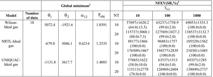
We use one data set for the system water-1,2 ethanediol at 430 mmHg. This system was also analyzed by Gau et al. (2000) using the least squares formulation and they reported several local optimums for the objective function. Also, they indicated that global optimal parameters provide a better fit to the experimental data. We optimize Eq. 11 with respect to the energy parameters of the Wilson, NRTL and UNIQUAC models. The energy parameters for the NRTL and UNIQUAC equations are defined as in DECHEMA. We use the same initial intervals employed in the last example for the Wilson model, while the feasible domain for the NRTL and UNIQUAC parameters are θ θ ∈1, 2 (-2000, 5000) and
12
α ∈(0.01, 10) and θ θ ∈1, 2 (-5000, 20000), respectively. These domains include the parameters reported in DECHEMA. Our results are presented in Table 3 and the statistical analysis is reported in Table 2. For the Wilson and UNIQUAC models, the parameter TSA and the interaction TSA – NT show a
significant statistical effect on the reliability of the data-fitting procedure. Also, SA shows some failures in the global minimization of the objective function. The global minimum reported for the Wilson model is in agreement with that published by Gau et al. (2000). The energy parameters reported in DECHEMA correspond to local optimums for the three models. Similar findings with other systems have been reported by Dominguez et al. (2002) using the Wilson and UNIQUAC equations.
Table 3: Results of parameter estimation for the water-1,2 ethanediol system at 430 mmHg using simulated annealing with the least squares formulation
NFEV(SR,%)1
Global minimum2
SA T
Model Number
of data θ1 θ2 α12 Fobj NT 10 100 1000
Wilson-Ideal gas
18
5072.4 -1921.6 1.0391 10 57697±1620.2 (64.0±13.5)
63237±1758.9 (99.0±2.0)
69053±1335.3 (100.0±0.0)
20 115737±3068.1
(80.0±7.3)
127569±2437.2 (99.0±2.0)
138537±3132.7 (100.0±0.0) NRTL-Ideal
gas -679.0 3046.1 0.6214 1.2535 10
88177±1866 (100±0.0)
96883±1757 (100±0.0)
105529±1562 (100±0.0)
20 176509±3467
(100±0.0)
194377±2839 (100±0.0)
210301±3485 (100±0.0)
UNIQUAC-Ideal gas -1131.8 3617.7 1.4085 10
57685±1622 (58.0±10.0)
63537±1513 (94.0±5.0)
69357±1285 (99.0±2.0)
20 115113±2778
(78.0±8.0)
126969±2604 (100.0±0.0)
138049±2737 (100.0±0.0)
1NFEV is defined as the average number of objective function evaluations during the optimization procedure and SR is the
success rate in finding the global minimum based on 4 groups of 25 calculations with random initial values and number seeds.
2 Global optimum is consistent with the results reported by Gau et al. (2000).
Problem 3. Benzene-Hexafluorobenzene (LS Formulation)
The parameter estimation of this problem is performed assuming VLE data under isothermal and isobaric conditions. This system has also been analyzed by Gau et al. (2000) using interval analysis. Four data sets are used to test the numerical performance of the SA method. We use a least squares formulation in the parameter estimation and the same initial intervals as those for the energy parameters of the Wilson model are applied. The results of parameter estimation are reported in Table 4, while the statistical analysis appears in Table 2. In this example, SA has a better numerical performance; however, it still shows some failures in the global minimum of the objective function. Only
for the data at 760 mmHg, SA finds the global minimum with a reliability of 100% and its numerical performance is independent of the values for parameters TSA and NT. We find a significant statistical effect of parameter NT in the reliability of the parameter estimation procedure for the data at 30 °C, 50 °C and 300 mmHg. For the case of TSA, it
Table 4: Results of parameter estimation for the benzene-hexafluorobenzene system using simulated annealing with the least squares formulation
NFEV(SR,%)1
Global minimum2
SA T
T, °C or P, mm Hg
Number
of data θ1 θ2 Fobj NT 10 100 1000
T = 30 10 -467.8 1313.9 0.0118 10 57841±1345.4 (91.0±8.9)
63569±1523.1 (96.0±3.3)
69081±1308.2 (100.0±0.0) 20 116105±2559.4
(99.0±2.0)
126833±2581.5 (100.0±0.0)
138449±3124.0 (100.0±0.0) 50 11 -424.1 983.1 0.0089 10 57745±1216.1
(97.0±2.0)
63413±1284.5 (100.0±0.0)
68957±1588.7 (100.0±0.0) 20 115929±2647.4
(100.0±0.0)
127337±2446.8 (100.0±0.0)
138649±2329.5 (100.0±0.0) P = 300 17 -432.5 992.9 0.0149 10 58097±1315.2
(89.0±6.0)
63501±1264.1 (95.0±5.0)
69177±1277.4 (96.0±3.3) 20 115505±2873.8
(97.0±3.8)
126937±2881.2 (99.0±2.0)
138481±2868.7 (99.0±2.0) 760 29 -334.7 704.7 0.0146 10 57901±1262.8
(100.0±0.0)
63641±1270.6 (100.0±0.0)
69217±1378.5 (100.0±0.0) 20 115673±2580.7
(100.0±0.0)
126977±2950.0 (100.0±0.0)
138209±2961.0 (100.0±0.0)
1NFEV is defined as the average number of objective function evaluations during the optimization procedure and SR is the
success rate in finding the global minimum based on 4 groups of 25 calculations with random initial values and number seeds.
2Global optimums are consistent with results reported by Gau et al. (2000).
Problem 4. Benzene-Hexafluorobenzene (EIV Formulation)
In this problem, we consider the modeling of vapor-liquid equilibrium of the binary system benzene-hexafluorobenzene using the error-in-variable approach. This system was studied by Gau and Stadtherr (2002) using interval analysis. Four data sets are used and parameter estimation is considered using the Wilson equation for liquid-phase activity coefficients. The state variables are (x , y , P, T1 1 ) where P is the system pressure in mmHg, T is the system temperature in °C and x1 and y1 are the liquid and vapor mole fractions of benzene. In accordance with Gau and Stadtherr (2002), a standard deviations of 0.001, 0.01, 0.75 and 0.1 are assumed for these variables. The vapor-liquid equilibrium can be described by the following equations
0 0
1 1 1 2 1 2
P= γ x P + γ (1−x )P (12)
0 1 1 1
1 0 0
1 1 1 2 1 2
x P y
x P (1 x )P
γ =
γ + γ − (13)
We formulate the data-fitting problem as unconstrained optimization using Eqs. [12] and [13]
to eliminate P and y1 from the objective function. For the unconstrained problem, the independent state
variables are the set of →z= x , T→ →1
for all
measurements, while the optimization variables are
(
)
T1, 2
→
θ = θ θ and the set of t t t
1
z x , T
→ → →
=
. The
objective function is defined as
(
) (
)
(
) (
)
1 1
2 2
t t
1i 1i 1i 1i
2 2
ndat x y
obj
2 2
t t
i 1
i i i i
2 2
T P
x x y y
F
T T P P
=
− −
+ +
σ σ
=
− −
+ +
σ σ
∑
(14)This function is optimized with respect to 2+2ndat variables where ndat is the number of experimental data used in parameter estimation. The initial intervals of the independent state variables are set using plus and minus three standard deviations, while the intervals for the Wilson model parameters
are defined as θ ∈ −1 ( 8500, 320000) and
2 ( 8500, 320000)
θ ∈ − . The results of parameter
analysis appears in Table 2. Due to the increase in problem dimensionality, SA fails several times in finding the global minimum for all data sets. For only two cases, it shows 100% reliability in the global minimization of the objective function. Also, there is a significant increase in the computational effort of the data-fitting procedure, also caused by problem dimensionality. Of course, we can reduce the numerical effort of the SA method by decreasing the tolerance
value and using a local search method to refine the solution obtained by SA. On the other hand, the variance analysis indicates that parameter TSA affects
the reliability of parameter estimation for all data sets. For data at 760 mmHg, NT has a significant effect on the success rate for finding the global optimum. An increase in both TSA and NT improves the reliability of
SA. The global optimums reported for all data are consistent with the results of Gau and Stadtherr (2002).
Table 5: Results of parameter estimation for the benzene-hexafluorobenzene system using simulated annealing with the error-in-variable formulation
NFEV(SR,%)1
Global minimum2
SA T
T, °C or P, mm Hg
Number
of data θ1 θ2 Fobj NT 10 100 1000
T = 50 11 -460.6 1115.8 19.525 10 756481±8521.0 (45.0±3.8)
826609±8081 (52.0±12.7)
896209±7906 (49.0±11.9) 20 1510177±15659.0
(46.0±5.2)
1652353±13867 (53.0±11.9)
1787041±13602.0 (69.0±8.3) 70 9 -424.2 1006.8 8.503 10 867401±326470
(58.0±10.1)
965961±347410 (55.0±7.6)
994281±401374 (62.0±10.6) 20 1534081±361615
(60.0±8.6)
1756321±616201 (58.0±10.6)
1645041±349990 (78.0±10.6) P = 300 17 -478.3 1118.7 37.399 10 1157689±18171
(54.0±5.2)
1259281±19591 (56.0±5.7)
1360297±19289 (59.0±6.0) 20 2296225±19676
(55.0±5.0)
2502865±17570 (56.0±5.7)
2709073±20534 (66.0±6.9) 760 29 -420.7 1060.3 16.925 10 4998841±3331470
(43.0±8.3)
4512481±2949822 (52.0±19.9)
4312441±3148616 (65.0±7.6) 20 4105201±1095049
(96.0±3.3)
4236001±32451 (100.0±0.0)
4567861±32340 (100.0±0.0)
1NFEV is defined as the average number of objective function evaluations during the optimization procedure and SR is the
success rate in finding the global minimum based on 4 groups of 25 calculations with random initial values and number seeds.
2Global optimums are consistent with results reported by Gau and Stadtherr (2002).
Problem 5. Methanol-1,2 Dichloroethane
This system was studied by Esposito and Floudas (1998) using a deterministic global optimization method. We consider the EIV parameter estimation using the van Laar model for liquid phase. The experimental data consists of five points for the state variables: pressure in mmHg, temperature in Kelvin and liquid and vapor mole fractions of methanol. The vapor pressure of pure components is calculated using
0 1
i 1
1 b
P exp a
T c
= −
−
(15)
where Pi0 is given in mmHg, T is given in Kelvin and the constants of the Antoine equation are taken
from Esposito and Floudas (1998). The activity coefficients are defined by
2 1 1
2 x
A A
exp 1
RT B x
−
γ = +
(16)
2 2 2
1 x
B B
exp 1
RT A x
−
γ = +
(17)
temperature as
r r
A B
, RT RT
→
θ =
. The state variables
of the system are 1 1
r
T x , y , P,
T
and their standard
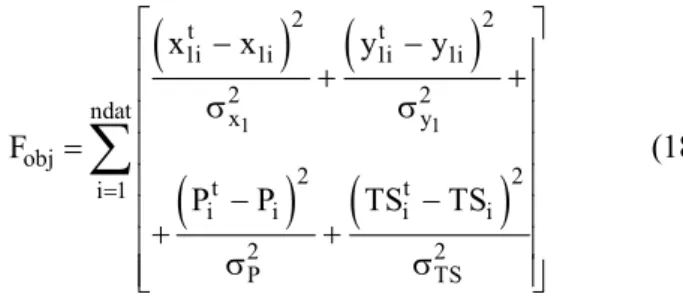
deviations are defined as 0.005, 0.015, 0.75 and 0.000309. The objective function is given by
(
) (
)
(
) (
)
1 1
2 2
t t
1i 1i 1i 1i
2 2
ndat x y
obj
2 2
t t
i 1
i i i i
2 2
P TS
x x y y
F
P P TS TS
=
− −
+ +
σ σ
=
− −
+ +
σ σ
∑
(18)whereTS=T / Tr. Equations [12] and [13] are used
to eliminate P and y1 in the objective function and we have twelve optimization variables where the initial intervals for the independent state variables
t t t
1 z x , T → → →
=
are set using plus and minus three
standard deviations. For the case of the van Laar
model parameters, we use
r
A
(1, 2)
RT ∈ and
r
B
(1, 2)
RT ∈ . The results of parameter estimation are
reported in Table 6. For all calculations performed, SA finds the global minimum of the objective function with 100% reliability. In this case, the parameters TSA and NT affect only the efficiency of
the data-fitting procedure. The global minimum reported is consistent with the results of Gau and Stadtherr (2002).
We have studied the numerical performance of SA with other examples reported by Gau et al. (2000) and Gau and Stadtherr (2002). The results obtained in those calculations, not reported here, indicate that SA is generally a reliable method for parameter estimation in VLE modeling.
Based on our experience with other SA algorithms, such as very fast simulated annealing (Sharma and Kaikkonen, 1999) and direct search simulated annealing (Ali et al., 2002), we can expect that the algorithm of Corana et al. (1987) has a better numerical performance and we consider it a suitable choice for data fitting in thermodynamic models.
Table 6: Results of parameter estimation for the methanol-1,2 dichloroethane system using simulated annealing with the error-in-variable formulation
NFEV(SR,%)1
Global minimum2
SA T
T, °C Number
of data r
A
RT r
B
RT Fobj NT 10 100 1000
50 5 1.912 1.608 3.326 10 370561±4435 (100.0±0.0)
404593±4766 (100.0±0.0)
438529±4370 (100.0±0.0)
20 742273±9166
(100.0±0.0)
810433±8783 (100.0±0.0)
878689±7863 (100.0±0.0)
1NFEV is defined as the average number of objective function evaluations during the optimization procedure and SR is the
success rate in finding the global minimum based on 4 groups of 25 calculations with random initial values and number seeds.
2Global optimum is consistent with results reported by Gau and Stadtherr (2002).
CONCLUSIONS
The numerical performance of the simulated annealing method has been tested in parameter estimation for VLE modeling. The reliability and efficiency of the data-fitting procedure was evaluated with respect to the SA parameters TSA and NT, using
classical least squares and error-in-variable formulations. Our results indicate that parameter TSA
significantly affects the reliability of the data-fitting procedure. On the other hand, both parameters affect the efficiency of the SA method. The SA method has a better numerical performance using the classical
least squares instead of the error-in-variables formulation. In general, SA is a robust optimization procedure, when properly implemented for parameter estimation using both formulations. However, it can fail in the global minimization of difficult systems.
ACKNOWLEDGMENTS
NOMENCLATURE
A, B parameters of the van Laar model
1 1 1
a , b , c parameters of the Antoine equation
NT iteration number before temperature
reduction
P Pressure 0
i
P vapor pressure of pure component
T temperature
SA
T annealing temperature
r
T reference temperature
1
x , y1 liquid and vapor mole fraction
ij
y dependent response variable
t ij
z unknown “true” value of state variable
i
σ standard deviation of state variable
1
θ , θ2 energy parameters
γ activity coefficient
REFERENCES
Ali, M.M., Törn, A., and Viitanen, S., A direct search variant of the simulated annealing algorithm for optimization involving continuous variables. Computers & Operations Research, 29 (1), 87-102 (2002).
Anderson, T.F., Abrams, D.S., and Grens, E.A. II., Evaluation of parameters for nonlinear thermodynamics models. AIChE Journal, 24 (1), 20-29 (1978).
Bard, Y., Nonlinear parameter estimation, Academic Press, New York (1974).
Britt, H.I., and Luecke, R.H., The estimation of parameters in nonlinear implicit models. Technometrics, 15, 233-247 (1973).
Corana, A., Marchesi, M., Martini, C., and Ridella, S., Minimizing multimodal functions of continuous variables with the simulated annealing algorithm. ACM Transactions on Mathematical Software, 13 (3), 262-280 (1987).
Costa, A.L.H., da Silva, F.P.T., and Pessoa, F.L.P., Parameter estimation of thermodynamic models for high-pressure systems employing a stochastic method of global optimization. Brazilian Journal of Chemical Engineering, 17 (3), 349-353 (2000).
Dominguez, A., Tojo, J., and Castier, M., Automatic implementation of thermodynamic models for reliable parameter estimation using computer algebra. Computers and Chemical Engineering, 26 (10), 1473-1479 (2002).
Englezos, P., and Kalogerakis, N., Applied parameter estimation for chemical engineers, Marcel-Dekker, New York (2001).
Esposito, W.R., and Floudas, C.A., Global optimization in parameter estimation of nonlinear algebraic models via the error-in-variables approach. Ing. Eng. Chem. Res., 37 (5), 1841-1858 (1998).
Fabries, J., and Renon, H., Method of evaluation and reduction of vapor-liquid equilibrium data of binary mixtures. AIChE Journal, 21 (4), 735-743 (1975).
Gau C.Y., Brennecke J.F., Stadtherr M.A., Reliable nonlinear parameter estimation in VLE modeling. Fluid Phase Equilibria, 168 (1), 1-18 (2000). Gau, C.Y., and Stadtherr, M.A., Deterministic global
optimization for error-in-variables parameter estimation. AIChE Journal, 48 (6), 1192-1197 (2002).
Gmehling, J., Onken, U., and Arlt, W., Vapor-liquid Equilibrium Data Collection, Chemistry Data Series, Vol. I, Parts 1-8, DECHEMA (1977-1990).
Goffe, B., Ferrier, G., and Rogers, J., Global optimization of statistical functions with simulated annealing. Journal of Econometrics, 60 (1-2), 65-99 (1994).
Henderson, N., de Oliveria, J.R., Amaral Souto, H.P., and Pitanga Marques, R., Modeling and analysis of the isothermal flash problem and its calculation with the simulated annealing algorithm. Ind. Eng. Chem. Res., 40 (25), 6028-6038 (2001).
Kirkpatrick, S., Gelatt, C., and Vecchi, M.P., Optimization by simulated annealing. Science, 220 (4598), 671-680 (1983).
Kleiber, M., and Axmann, J.K., Evolutionary algorithms for the optimization of modified UNIFAC parameters. Computers and Chemical Engineering, 23 (1), 63-82 (1998).
Metropolis, N., Rosenbluth, A., Rosenbluth, M., Teller A., and Teller, E., Equation of state calculations by fast computing machines. J. Chem. Phys., 21 (6), 1087-1092 (1953).
Michalewicz Z., Fogel D.B., How to solve it? Modern heuristics, Springer (1999).
Park, T.Y., and Froment, G.F., A hybrid genetic algorithm for the estimation of parameters in detailed kinetic models. Computers and Chemical Engineering, 22 (S1), S103-S110 (1998).
Reid, R.C., Prausnitz, J.M., and Sherwood, T.K., The properties of gases and liquids, 3rd Ed., McGraw-Hill, New York (1987).
Sharma, S.P., and Kaikkonen, P., Global optimisation of time domain electromagnetic data using very fast simulated annealing. Pure and Applied Geophysics, 155 (1), 149-168 (1999). Tjoa, T.B., and Biegler, L.T., Reduced successive
quadratic programming strategy for
errors-in-variables estimation. Computers Chemical Engineering, 16 (6), 523-533 (1992).
Valko, P., and Vajda, S., An extended marquardt-type procedure for fitting error-in-variables methods. Computers Chemical Engineering, 11 (1), 37-43 (1987).