Braz. J. Chem. Eng. vol.24 número1

ISSN 0104-6632 Printed in Brazil

www.abeq.org.br/bjche

Vol. 24, No. 01, pp. 119 - 133, January - March, 2007

Brazilian Journal

of Chemical

Engineering

A KINETIC MODEL FOR THE FIRST STAGE

OF PYGAS UPGRADING

J. L. de Medeiros

, O. Q. F. Araújo

, A. B. Gaspar

, M. A. P. Silva

and J. M. Britto

1

Escola de Química, Universidade Federal do Rio de Janeiro, Centro de Tecnologia, Bl. E, Phone (+55) (21) 2562-7535, Ilha do Fundão, 21949-900, Rio de Janeiro - RJ, Brazil

Email: jlm@eq.ufrj.br

2

BRASKEM S.A., Planta de Insumos Básicos, Phone (+55) (71) 632-5809, Rua Eteno 1561, 42810-000, Polo Petroquímico, Camaçari - BA, Brazil.

Email: jaildes@braskem.com.br

(Received: March 28, 2005 ; Accepted: October 31, 2006)

Abstract - Pyrolysis gasoline – PYGAS – is an intermediate boiling product of naphtha steam cracking with a high octane number and high aromatic/unsaturated contents. Due to stabilization concerns, PYGAS must be hydrotreated in two stages. The first stage uses a mild trickle-bed conversion for removing extremely reactive species (styrene, dienes and olefins) prior to the more severe second stage where sulfured and remaining olefins are hydrogenated in gas phase. This work addresses the reaction network and two-phase kinetic model for the first stage of PYGAS upgrading. Nonlinear estimation was used for model tuning with kinetic data obtained in bench-scale trickle-bed hydrogenation with a commercial Pd/Al2O3 catalyst. On-line sampling experiments were designed to study the influence of variables – temperature and spatial velocity – on the conversion of styrene, dienes and olefins.

Keywords: Hydrotreatment Hdt; Pygas; Trickle bed; Kinetic model.

INTRODUCTION

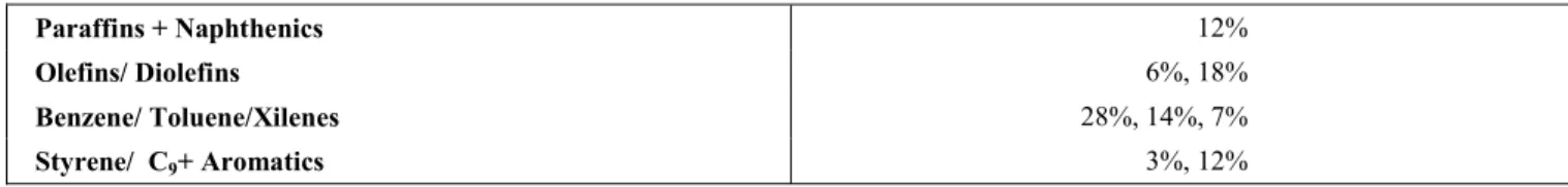
Naphta steam cracking is the most frequently used process for production of high-value petrochemical olefins like ethylene and propylene (Edwin, 1994). The main byproduct of this process is an intermediate boiling-point fraction known as pyrolysis gasoline or PYGAS. PYGAS has high aromatic and unsaturated contents, with typical

weight composition shown in Table 1.

The increasing global trend to process heavier – and cheaper – feedstocks for light olefin production poses the problem of the increasing need to utilize liquid byproducts, like PYGAS (Cheng et al., 1986). PYGAS, on the other hand, offers the option of processing to yield high-octane blending mixtures and C6-C8 cuts suitable for extraction of aromatics.

Table 1: Typical Weight Composition of PYGAS

Paraffins + Naphthenics 12%

Olefins/ Diolefins 6%, 18%

Benzene/ Toluene/Xilenes 28%, 14%, 7%

Ordinary PYGAS is a very unstable liquid due to the presence of large amounts of unsaturated or polyunsaturated species (Table 1). In order to guarantee stabilization for subsequent processing, it must be hydrotreated (Cosyns, 2000) to destroy its extremely reactive species – like styrene, olefins and dienes – and other undesirable sulfured compounds. This hydrotreatment process (HDT) occurs in two stages at pressures near 30 bar. The first stage is conducted under milder conditions in a trickle-bed cocurrent downflow (Ragaini and Tine, 1984) reactor filled with a Pd/Al2O3 catalyst. This stage is

designed to convert most of the styrene, aliphatic dienes (e.g. octadienes) and cyclic dienes (e.g. dicyclopentadiene, DCPD) under controlled conditions in order to prevent gum and coke formation over the bed. The temperature and weight hourly spatial velocity (WHSV) ranges are from 50oC to 130oC and from 1.5h-1 to 5h-1, respectively. The effluent PYGAS from the first stage is then vaporized and sent to the second stage where a more severe, gas-phase hydrogenation takes place, aiming at complete conversion of unsaturated and sulfured species at temperatures above 200oC. It is vital that no appreciable quantity of dienes or styrene reach the second stage; otherwise gum formation followed by coke deposition will take place, fouling the CoMo/alumina bed.

As can be seen, PYGAS upgrading is only an auxiliary process in a complex olefin plant. Its costs are, nevertheless, seriously relevant. This is a consequence of H2 recycling and compression as

well as of high catalyst inventories – as usual, submitted to aging and deactivation processes – and heavy use of thermal utilities (Cosyns, 2000). In other words, a good modeling of these reactive operations is needed in order to enable reliable simulation and optimization of the process, thus allowing the exploration of more profitable, i.e. less costly or more durable, operational runs.

Previous (and public) studies addressing kinetic modeling of PYGAS upgrading are scarce. Some useful results can be found in the work of Cheng et al. (1986). These authors present characterization data on typical PYGAS streams and kinetic data for the conversion of model compounds isoprene and styrene in a batch reactor for temperatures ranging from 60oC to 180oC and pressures between 20 and 50 bar. Their results were expressed as irreversible first order kinetic laws in terms of liquid-phase concentrations of reactant hydrocarbon and dissolved hydrogen. Arrhenius plots of kinetic constants against the inverse of temperature were also

presented.

Using experimental data supplied by Cheng et al. (1986) on physical characterization of a typical crude PYGAS, Cardoso et al. (2002) developed and fitted a compositional model for this fraction. This model was built with 18 molecular lumps and three independent molecular growth terms via lateral paraffinic chains formulated according to the rules proposed by Quann and Jaffe (1996) and also implemented, in several different hydrotreatment (HDT) scenarios, by Barbosa et al. (2002), Costa et al. (2002), Vargas et al. (2002) and de Medeiros et al. (2002, 2004). The PYGAS compositional model and the kinetic constants presented by Cheng et al. (1986) were then used to generate pseudo-experimental characterization data for a typical series of isothermal hydrogenation runs of PYGAS. Finally, this set of pseudo-measured characterization of hydrogenated products was used to estimate kinetic and adsorption parameters for a proposed reaction network appropriate for the first stage of PYGAS hydrotreatment (Cardoso et al., 2002). Though barely supported by true experimental information, the purpose of the work of Cardoso et al. (2002) was to present a complete methodology to treat characterizing data generated by pilot/bench hydrogenation runs of PYGAS, aiming at the development of a physically sound industrial reactor model for this process.

An alternate strategy for developing models on hydrotreatment (HDT) of complex feeds consists of separate kinetic studies covering individually each one of the most relevant classes of chemical reactions that takes place. In this case, one chooses a set of reactant and inert model compounds from which synthetic feeds are prepared for hydrogenation runs following a careful experimental design. This was the case in the work of Gaspar et al. (2003), which presented results on estimation of Arrhenius parameters – K0 and EATIV – for four kinetic laws and

component adsorption constants – KADS – of a

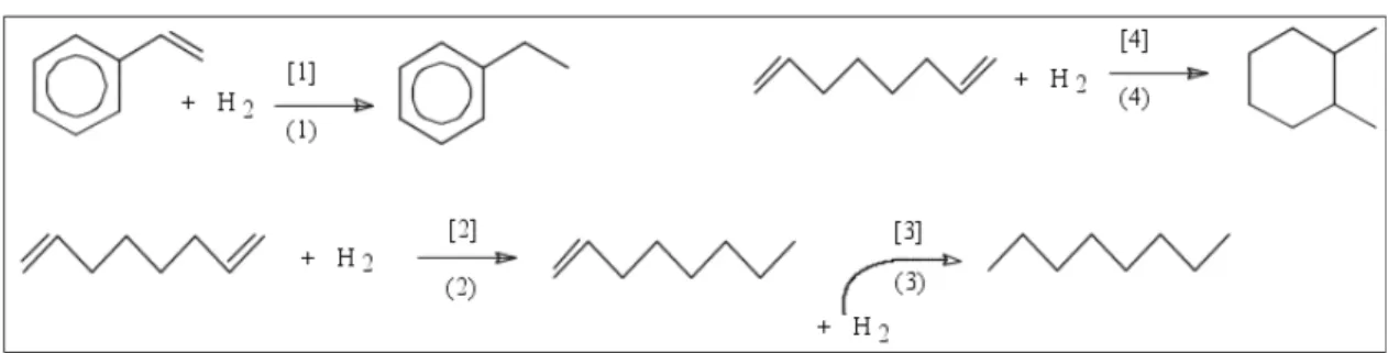
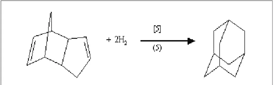
Figure 1: Hydrogenation Reaction Network (Gaspar et al., 2003)

The present work extends the Gaspar et al (2003) results in three directions. First, new experiments with synthetic feeds were conducted, totaling 120 hydrogenating (HDT) runs with temperature ranging between 35 and 100 oC and WHSV ranging between 2 and 70 h-1. Second, the reaction network was extended via insertion of DCPD into the set of reactant model compounds, so that there is a new reaction accounting for the full hydrogenation of DCPD into adamantane (tetrahydroDCPD). Third, due to a more comprehensive survey of experimental data, the estimation procedure now used was based on nonlinear estimation of kinetic and adsorption constants for five slices of nearly isothermal runs, extracted from the database for temperatures of 40oC, 50oC, 60oC, 70oC and 100oC. With the corresponding five sets of estimated parameters, Arrhenius coefficients can be easily produced through linear regression on a logarithmic scale versus the inverse of absolute temperature.

EXPERIMENTAL PROCEDURE

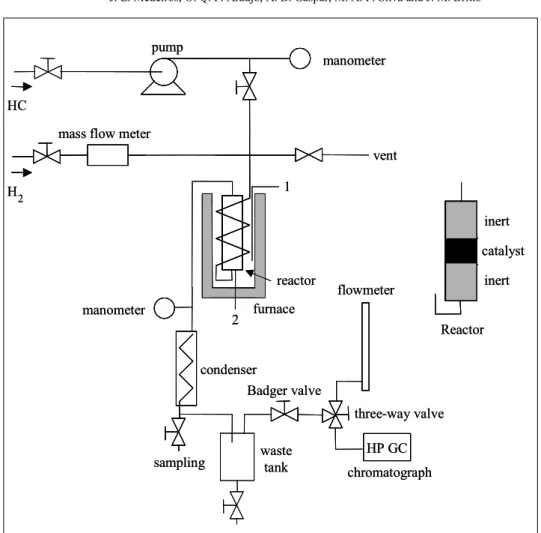
Experiments on hydrogenation of model compounds were conducted in a continuous bench plant with an up-flow fixed bed reactor, as explained in Gaspar et al. (2003) and shown in Figure 2. The unit operates under approximately steady conditions through continuous pumping of liquid reactant (HC in Figure 2) and hydrogen. Reactor discharge pressure is tightly controlled via a Badger valve under PID control. The reactor stainless steel chamber has a length of 20 cm and an inside diameter of 2.54 cm, warranting a chamber/particle diameter ratio greater than 8, which is necessary to minimize bad hydrodynamic effects (Mears, 1971a,b). All experiments used the same commercial Pd/Al2O3 catalyst as before (0.3wt% Pd). The

catalyst bed was made of approximately 1g of catalyst beads dispersed in inert ceramic beads (1:1 ratio) to ensure homogeneous distribution of feed and to avoid local overheating. Reactor temperature

was kept fixed through an electrical furnace operated by a PID temperature controller having a thermocouple axially posed in the center of the bed. In order to fill up the reactor, inert beads were introduced before and after the catalyst bed, as shown in Figure 2. Before each run, the catalyst was reduced with hydrogen (30 Ncm3/min) at 130 oC for 2 hours (bed temperature increasing at 10

o

C/min) under atmospheric pressure.

The reactor inlet receives a two-phase stream of H2

mixed with liquid hydrocarbon feed at controlled temperatures (T), pressures (P), H2/Feed ratios and

mass flow meter

waste tank sampling

H 2

vent pump

manometer

reactor

furnace manometer

condenser

HP GC Badger valve

three-way valve flowmeter

chromatograph 1

2 HC

catalyst inert

inert

Reactor mass flow meter

waste tank sampling

H 2

vent pump

manometer

reactor

furnace manometer

condenser

HP GC Badger valve

three-way valve flowmeter

chromatograph 1

2 HC

catalyst inert

inert

Reactor

Figure 2: Schematic Representation of Experimental Plant (1 and 2 are temperature sensors)

Different hydrocarbon feeds were prepared, always using toluene as the solvent. A total of 15 valid experiment feeds were processed in this study, labeled sequentially as 4, 5, 6, 7, 8, 9, 10, 12, 13, 14, 15, 16, 17, 18 and 19. In each feed, reactant species compositions near the corresponding values in real PYGAS were chosen. Several binary feeds were formulated with styrene, DCPD or 1,7-octadiene as solute. Quaternary feeds were prepared with styrene, 1-octene and 1,7-octadiene as solutes, whereas five component feeds also included DCPD. Each feed gave rise to a group of runs for T between 35 and 100 oC and WHSV between 2 and 70 h-1 according to two-dimensional factorial designs (square-star or central composite design) with two or three replicas at the central point (Douglas, 1997). Total pressure (P) in each run was set at 30 bar (minimum of 28 bar, maximum of 38 bar). H2/Feed ratios were set

preferentially at 132 Nl/kg, though some low values were also employed (minimum of 24 Nl/kg, maximum of 137 Nl/kg). It must be pointed out that

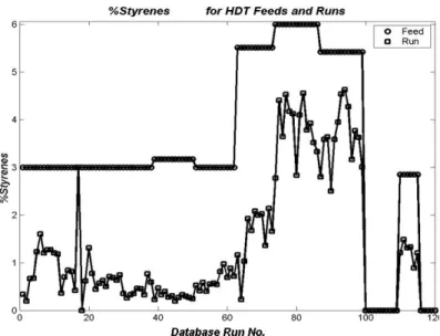
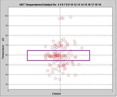
these ranges of experimental coordinates were chosen so that typical industrial process conditions were covered by the experimental cloud. Figure 3 shows the distribution of experimental coordinates along the database with 120 hydrogenation runs. Valid experimental coordinates are WHSV(h-1), T(oC), P(bar), H2/Feed(Nl/kg), feed composition and

catalyst type. For conciseness reasons, feed composition will be reported jointly with experimental responses. In all runs the above-mentioned Pd/Al2O3

catalyst was referred to as Catalyst 1. H2 consumption

was not recorded (Figure 3). The corresponding distribution of feeds is depicted in Figure 4.

Figure 3: Distribution of Experimental Coordinates for the Database of HDT Runs

Figure 4: Distribution of Hydrocarbon Feeds for the Database of Experiments

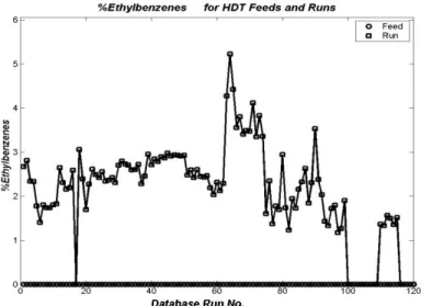
Figure 6: Distribution of wt% of Ethylbenzene for Feeds and Runs in the Experimental Database

Figure 7: Distribution of wt% of 1,7-Octadiene for Feeds and Runs in the Experimental Database

REACTION NETWORK AND KINETIC MODEL

The extended (irreversible) reaction network used is composed of the set of reactions (indexed with (.)) and kinetic rules (indexed with [.]) shown in Figure 1, complemented with the complete hydrogenation of DCPD to adamantane shown in Figure 9 –

reaction (5) and kinetic law [5]. These reactions are described by a kinetic model appropriate for simultaneous flow of liquid and gas reactive phases through a porous catalyst bed. Gas and liquid phases are assumed to be permanently at thermodynamic equilibrium inside the reactor. For all species Langmuir adsorption equilibria between the bulk phases and the catalyst (active) surface are assumed.

Figure 9: Hydrogenation of DCPD (Reaction No. 5, Kinetic Law No. 5)

In this study we neglect all heat/mass transfer resistances in model development. As verified in other experimental (Korre et al., 1997) and analytical (Martens and Marin, 2001) studies on heterogeneous hydroprocessing of hydrocarbons at high pressures, transport limitations are relatively unimportant for reaction modeling near industrial conditions of temperature, pressure and spatial velocity, which is precisely the case here. Kinetic rates are modeled with the following four-steps mechanism, where H2(g), Hσ(s), σ(s), HC(l), HCσ(s), HCσ-Hσ(s) and

HCHσ(s) are convenient representations of non-adsorbed hydrogen, dissociated hydrogen non-adsorbed on an active site, an unoccupied active site, non-adsorbed hydrocarbon, non-adsorbed hydrocarbon on an active site, hydrogenated unstable complex over catalyst, adsorbed hydrogenated species on an active site, respectively:

(1) equilibrium adsorption/dissociation of H2

[H2(g)+2σ(s)↔2Hσ(s)];

(2) equilibrium adsorption of hydrocarbon species [HC(l)+σ(s)↔HCσ(s)];

(3) slow reaction (order 1) of adsorbed species on catalyst [HCσ(s)+Hσ(s)→HCσ-Hσ(s)];

(4) fast subsequent hydrogenation [HCσ -Hσ(s)+nHσ(s)→HCHσ(s)+nσ(s)].

Taking into account the above considerations, and representing the equilibrium fugacity (in bar) of species i by fi, the rate (in gmol/s/kgcat) expression

for the kth reaction is written according to Eqs. (1) and (2) below:

AD

k k j j

R (T, f )=K (T) *Ψ(T, f ) * K * f (1)

AD

H2 H2

2

AD AD

H2 H2 j j

j H2 K (T) * f (T, f )

1 K (T) * f K (T) * f

≠

Ψ =

 

 + + 

 



∑

(2)

where Kk(T) is the kinetic constant of the k th

reaction having species j as the hydrocarbon reactant; Kj

AD

(T) is the adsorption (Langmuir) equilibrium constant (in bar -1) of species j. The column vectors

AD

R(T, f ), K(T), K (T) and f represent respectively nr reaction rates, nk kinetic constants, nc component adsorption constants and nc component equilibrium fugacities. We introduce also the matrices S and D ,

with sizes nr x nc and nr x nk, such that

kj

S = ⇒1 kth reaction rate is defined by species j, otherwise S_kj =0

ki

D = ⇒1 kth reaction rate uses ith kinetic law, otherwise D_ki =0

Then the vector of reaction rates for the entire network can be written according to Eq. (3):

(

)

(

)

R(T, f ) (T, f ) * Diag(DK(T)) *

S * K (T) f

= Ψ

•

(3)

0

K(T)=K •exp( E / T)− (4)

AD AD AD

0

K (T)=K •exp( E− / T) (5)

where E, EAD, K0 and K0 AD

express corresponding vectors of activation energies (in K), reference kinetic constants and reference Langmuir constants. The symbol • stands for multiplication of the corresponding components of vectors of same size. Spatial reactor time (in kgcat/kg/s) can now be

defined from reactor section area A(m2), spatial axial coordinate z(m), catalyst density ρcat(kg/m3) and hydrocarbon feed flow rate F0(kg/s), as shown in Eq.

(6). From previous definitions, nc stationary component material balances along the bed are written as shown in Eq. (7). In these formulae, N and

H express respectively the nc x 1 vector of

component molar rates (in gmol/s) and the nc x nr stoichiometric matrix for the network of chemical reactions.

cat 0

t=z * A *ρ / F (6)

0

AD

d

N F * (T, f ) * H * Diag dt

(DK(T)) * S * (K (T) f )

= Ψ

• (7)

Reactor (or experiment) responses can be produced by integration of the reactor ordinary differential equations (Eq. (7)), from t=0 to t=3600/WHSV, symbolically represented as shown in Eq. (8):

(

)

0 t 3600/ WHSV 0

t 0

AD

F * (T,f ) * H *

Diag(DK(T)) *S*

N N dt

(K (T) f )

=

=

Ψ

= +

•

∫

where Diag(.) is an operator that transforms a vector

into a diagonal matrix form and N0 is the vector of

component molar rates at the reactor inlet. N0 is

defined by F0, the current feed composition and the

corresponding H2/Feed ratio. Eq. (8) is numerically integrated with adaptive methods appropriate for stiff problems. Along all points on the integration path, successive vapor-liquid equilibrium problems with specified T, P and N – flash(T,P,N) – have to be solved via Newton-Raphson procedures.

Thermodynamic properties (e.g. component fugacity

coefficients_φˆVAP_{, φ}ˆLIQ_{) are calculated for both}

phases by Soave-Redlich-Kwong equation of state with classical mixing rules (Reid et al., 1987).

PARAMETER ESTIMATION

At a given temperature, the vector of np model parameters (θ) may be estimated with the corresponding (nearly) isothermal slice of database runs and responses. The estimate of θ is written as ˆθ. Vector ˆθ is composed of nk=5 kinetic constants and nc=10 component Langmuir constants

(θ =ˆT [KˆT KˆADT]). Each run i produced a ny x 1 vector of experimental responses Y_iEXP (see Experimental Procedure section) with ny=9. The predicted model responses for the same run – via Eq. (8) – are defined as Y ( )ˆ_i θˆ .

Let Y ( )ˆ_i θ −ˆ YEXP_i represents the vector of response residue for run i. Then, neglecting constant terms, the logarithmic likelihood function of run i may be represented by Eq. (9) below. In Eq. (9),

i

W is the ny x ny diagonal weighting matrix for run

i, which expresses some knowledge about the variance of random errors affecting experimental values (Eq. (10)). Eq. (10), in turn, introduces D% : a known vector of percent standard deviations assigned to experimental responses:

EXP T

i i i

EXP

i i

i

ˆ ˆ

ln(L ) ( 1/ 2)(Y ( ) Y )

ˆ ˆ

W (Y ( ) Y )

= − θ −

θ − (9)

1 EXP

i

i _EXP

i

Diag(D% Y /100)

W

Diag(D% Y /100)

−  _{• •}   =   •     (10)

bounded search on θ space through unbounded new η variables, as shown in Eq. (12):

m

EXP T EXP

i i _i i i

i

INF SUP

1 _{ˆ ˆ ˆ ˆ}

Min (Y ( ) Y ) W (Y ( ) Y ) 2

ˆ

{ }

  _{θ − θ −}

   

θ ≤ θ ≤ θ

∑

(11)

INF ( SUP INF)

(1 )

θ = θ + θ − θ •

•η • η • + η • η

(12)

STATISTICAL ANALYSIS

Several statistical entities are used for evaluation of the goodness of the estimation process. The analysis uses standard formulae if it can, cumulatively, be assumed that

(1) Experimental responses follow Gaussian distributions and are statistically independent;

(2) Experimental runs are statistically independent; (3) The reactor model gives a good description of the experiment;

(4) The optimum of Eq. (11) is found within the feasible region of parameter values.

Thus, statistics SR 2

, given by Eq. (13), is a valid estimator for the intrinsic problem variance. Accordingly, estimators for variance-covariance matrices for estimated parameters and predicted responses are shown respectively in Eq. (14) and (15). The correct parameter (joint) confidence region at level (1-α)*100% (α=0.01) can be estimated with Eq. (16). The correct parameter confidence intervals at level (1-α)*100% (α=0.01) can be estimated with Eq. (17). Confidence intervals of the correct responses of run i, at level (1-α)*100% (α=0.01), can be estimated with Eq. (18). In all these formulae some symbolic terms have to be defined:

( )

i i

ˆ

J = ∇_θY represents the Jacobian matrix of

responses of run i (Yˆ_i) with estimated parameters

(θ), [.]-1 is a symbolic representation of the matrix obtained according to

1 m

1 T

i i i i 1

[.] J W J

− − =   = _ _ 

∑

operator diag(.) produces columnar extraction of the

main diagonal of a matrix, φ1-α is the Fisher abscissa

for the chosen confidence level and (np, ny*m-np)

degrees of freedom, t_{1−α/ 2}is the t (Student) abscissa for the chosen confidence level and (ny*m-np) degrees of freedom.

2 R

m

EXP T EXP

i i _i i i

i

1 S

ny * m np

ˆ ˆ

(Y Y ) W (Y Y )

  =  ₋    − −

∑

T 2 1

R

i i i

i 1

ˆ ˆ

COV( ) S *

* J W J S *[.]

− − = θ =   =     

∑

i _{i i}

ˆ ˆ

COV(Y )= S * J [.] J− (15)

m T T

i i i

i 1

2

R 1

ˆ

( ) * J W J *

ˆ

*( ) np * S *

=

−α

 

θ − θ _ _

 

θ − θ ≤ φ

∑

(16)

1 2

1 / 2 R

1 2

1 / 2 R

ˆ _{t S * diag([.] )} ˆ

t S * diag([.] )

− −α

− +α

θ − ≤ θ ≤ θ+

+

(17)

1 T 2

1 / 2 R

i _{i i} i i

1 T 2

1 / 2 R _{i i}

ˆ ˆ

Y t S * diag(J [.] J ) Y Y

t S * diag(J [.] J )

− −α − +α − ≤ ≤ + + (18) ESTIMATION RESULTS

ensemble of runs on the temperature-catalyst plane. This slice has the highest number of runs (m=57), comprising experiments with temperatures between 54 oC and 64 oC. Percent standard deviation (D%) for all observed responses was assumed to be equal

to 10%. In the figures and tables that follow, species are coded as ST: styrene, EB: ethylbenzene, TOL: toluene, R=: 1-octene, R= =: 1,7-octadiene, R: n-octane, CR: 1,6dimethylcyclohexane, C= =: DCPD, C: adamantane and H2: hydrogen.

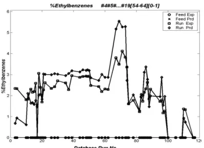
Figure 10: The Slice of Runs for Nominal Temperature of 60 oC In Figures 11, 12 and 13 the distribution of

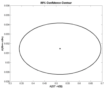
observed and estimated responses for wt% ethylbenzene, wt% 1,7-octadiene and wt% adamantane are presented. Only points belonging to the slice centered at T=60oC (Figure 10) are shown. Figure 14 is a two-dimensional projection of the 99% confidence region for kinetic parameters of styrene conversion (KST→EB) and conversion of 1,7-octadiene

into 1-octene (KR==→R=). In Figure 15 the same is

shown for the pair KR==→CR and KR=→R. In Table 2 a

summary of estimation results for this slice of data

(T=60oC) is presented. Finally, in Figure 16 a logarithmic plot of observed responses versus predicted ones is presented (the locus observed = predicted is shown as a dashed thick line). Due to its huge size, the corresponding legend of experimental coordinates is only partially shown (F:Feed No., T:Temperature, P:Pressure, W:WHSV, R:H2/feed). Figures 11, 12, 13 and 16 show on their top section the list of feeds followed by the temperature/catalyst ranges associated to the corresponding set of runs.

Table 2:Summary ofEstimation Results (T=60 oC)

Number of Runs : m=57 Number of Parameters : np=15

Responses per Run : ny=9 Confidence Level : α=0.99

D%=10% SR2=28.8

KST→EB

0.52

KR= =→R=

0.032

KR=→R

0.103

KR= =→CR

0.01

KC= =→C

1.99 KTol

AD

0.032

KST AD

0.063

KEB AD

0.014

KR= = AD

0.34

KR= AD

0.0014 KR

AD

0.40

KCR AD

0.042

KC= = AD

0.044

KC AD

0.087

KH2 AD

Figure 11: Observed Versus Predicted wt % Ethylbenzene (T=60 oC)

Figure 12: Observed Versus Predicted wt % 1,7-Octadiene (T=60 oC)

Figure 14: 2D Projection of 99% Confidence Region KR= =→R= Versus KST→EB (T=60 oC)

Figure 15: 2D Projection of 99% Confidence Region KR= =→CR Versus KR= →R (T=60

o

Figure 16: Logarithmic Plot of Observed Versus Predicted Responses (T=60 oC) [Partial Legend Showing F:Feed, T:Temperature, P:Pressure, W:WHSV, R:H2/feed]

With similar results prepared for the remaining slices of experiments (40oC, 50oC, 70oC and 100oC), independent Arrhenius linear regressions can be easily conducted for each kinetic/adsorption constant according to Eqs. (4) and (5).

CONCLUDING REMARKS

We developed a kinetic and reactor model for the first stage of PYGAS upgrading. The model was prepared from a database built with 120 hydrogenation runs of synthetic feeds made with five model compounds in the PYGAS reactive scenario. Though simple enough for engineering, our model takes into account important aspects like the two-phase (equilibrated) flow along the reactor and kinetic rates expressed with adsorption effects and component fugacities. Model parameters – five kinetic constants and ten Langmuir adsorption constants – were estimated at five temperatures via statistical processing of the corresponding five isothermal slices of experimental data using maximum likelihood techniques. Arrhenius forms for all these constants can be generated through linear regressions for the corresponding estimated values. These forms are useful for developing an engineering model of the (adiabatic) industrial reactor for PYGAS upgrading.

We presented detailed estimation results for the slice of experiments around T=60oC. Examining these results, it can be seen that some sectors of the reaction network were better adjusted than others. This was apparently the case for the kinetic law for hydroconversion of styrene into ethylbenzene (KST→EB) as compared with the kinetic law for

hydroconversion of DCPD into adamantane (KC==→C). The better fitting of the predicted

responses of wt% of ethylbenzene may be a consequence of the heavy dominance of ethylbenzene/styrene responses over DCPD/adamantane counterparts in the experimental database.

ACKNOWLEDGEMENTS

This work received financial support from FINEP/CTPETRO/BRAZIL, BRASKEM S.A. and CNPq/BRAZIL. The authors would like to express their gratitude to these institutions.

NOMENCLATURE

A Reactor section area (m2 )

COV(.) Variance-covariance matrix (-)

D% Vector of percent standard deviations of experimental

responses

D Matrix for assigning kinetic laws to reactions

(-)

Diag, diag Operators related to diagonal matrices

(-)

E, EAD Activation energies for kinetic and adsorption constants

(K)

F0 Mass flow rate of

hydrocarbon fed into reactor

(kg/s)

f Equilibrium component

fugacities

(-)

H Stoichiometric matrix for reaction network

(-)

i

J Jacobian matrix of predicted responses of run i with model parameters

(-)

K, KAD Vectors of kinetic and adsorption constants

(gmol/s kgcat,

bar-1) K0 ,

K0

AD Vectors of kinetic and

adsorption reference constants

(gmol/s kgcat,

bar-1)

Li Likelihood function of run i (-)

m Number of runs in an

isothermal slice of runs

(-)

nc, nr, nk Numbers of components, chemical reactions and kinetic laws

(-)

np, ny Numbers of parameters and model responses

(-)

N, N0 Vectors of component molar

rates

(gmol/s)

P Pressure (bar)

R Vector of reaction rates (gmol/s kgcat)

S Matrix for assigning

(hydrocarbon) reactant species to reactions

(-)

SR 2

Weighted sum of squared residuals

(-)

t Reactor spatial time (kgcat/kg/s)

t1-α/2 Student abscissa for

confidence level

(1-α)*100%

T Temperature (K)

i

W Weighting matrix for run i (-)

WHSV Reactor spatial velocity (kg/h/kgcat)

EXP

i i

ˆ

Y , Y Vectors of predicted and observed responses for run i

(-)

Yi Vector of correct responses

for run i

(-)

z Reactor axial position (m)

α Parameter for defining

confidence level

(α=0.01)

cat

ρ Density of catalyst bed (kg/m3)

ˆ ,

θ θ Vectors of correct and estimated model parameters

(-)

(T, f )

Ψ Adsorption term defined by

Eq. (2)

(-)

REFERENCES

Barbosa, L.C., Vargas, F.M., de Medeiros, J.L., Araujo, O.Q.F., da Silva, R.M.C., Modelagem de Hidrotratamento de Óleos Bases de Lubrificantes, Proceedings XIV COBEQ 2002, Natal, Brazil (2002).

Britt, H.I. and Luecke, R.H., The Estimation of Parameters in Nonlinear Implicit Models, Technometrics, 5, No. 2, 233 (1973).

Cardoso, R.M., de Medeiros, J.L., Araújo, O.Q.F., da Silva, M.A.P., Modelagem Cinética para Hidrogenação de Espécies de Gasolina de Pirólise, Proceedings XIV COBEQ 2002, Natal, Brazil (2002)

Cheng, Y.M., Chang, J.R., Wu, J.C., Kinetic Study of Pyrolysis Gasoline Hydrogenation over Supported Palladium Catalyst, Appl. Cat., No. 24, 273 (1986).

Costa, F.D., de Medeiros, J.L., da Silva, M.A.P., Araujo, O.Q.F., Leiras, A., Modelagem Composicional de Frações Leves de Petróleo via Curva de Destilação Simulada, Proceedings XIV COBEQ 2002, Natal, Brazil (2002).

Cosyns, J., Quicke, L., Debuisschert, Q., Pygas Upgrading, IFP (2000).

de Medeiros, J.L., Araújo, O.Q.F., da Silva, R.M.C., A Compositional Framework for Feed Characterization Applied in the Modeling of Diesel Hydrotreating Processes, Proceedings 17THWPC World Petroleum Congress, Rio de Janeiro, Brazil (2002).

de Medeiros, J.L., Barbosa, L.C., Vargas, F.M., Araujo, O.Q.F., da Silva, R.M.F., Flowsheet Optimization of a Lubricant Base Oil Hydrotreatment Process, Braz. J. of Chem. Eng., 21, No. 2, 317 (2004)

Douglas, M.C., Design and Analysis of Experiments, 5th Ed., John Wiley (1997).

Edwin, E.H., Modeling, Model Based Control and Optimization of Thermal Cracking and Ethylene Production, Dr.Ing. Thesis, Trondheim, Technology Norwegian Inst. (1994).

Korre, S.C., Klein, M.T., Quann, R.J., Hydrocracking of Polynuclear Aromatic Hydrocarbons: Development of Rate Laws through Inhibition Studies, Ind. Eng. Chem. Res., 36, 2041 (1997). Martens, G.G., Marin, G.B., Kinetics for

Hydrocracking Based on Structural Classes : Model Development and Application, AIChE Journal, 47, No. 7, 1607 (2001).

Mears, D.E., The Role of Axial Dispersion in Trickle Flow Laboratory Reactors, Chem. Eng. Sci., 26, 1361 (1971a).

Mears, D.E., Test for Transport Limitations in Experimental Catalytic Reactors, Ind. Eng. Chem. Process Des. Dev., 10, 541 (1971b).

Quann, R.J., Jaffe, S.B., Building Useful Models of Complex Reaction Systems in Petroleum

Refining, Chem. Eng. Sci., 51, No. 10, 1615 (1996).

Ragaini, V., Tine, C., Upflow Reactor for Selective Hydrogenation of Pyrolysis Gasoline – A Comparative Study with Respect to Downflow, Appl. Cat., No. 10, 43 (1984).

Reid, R.C., Prausnitz, J.M., Poling, E., The Properties of Gases and Liquids, 4th Ed., Mcgraw-Hill, N.Y. (1987)

Reklaitis, G.V., Ravindran, A., Ragsdell, K.M., Engineering Optimization, J. Wiley & Sons (1983). Vargas, F.M., Barbosa, L.C., de Medeiros, J.L.,