ISSN 0104-6632 Printed in Brazil
www.abeq.org.br/bjche
Vol. 26, No. 03, pp. 545 - 554, July - September, 2009
*To whom correspondence should be addressed
Brazilian Journal
of Chemical
Engineering
MODELING AND SIMULATING THE DRYING OF
GRASS SEEDS (Brachiaria brizantha) IN
FLUIDIZED BEDS: EVALUATION OF HEAT
TRANSFER COEFFICIENTS
A. C. Rizzi Jr., M. L. Passos and J. T. Freire
*Programa de Pós-Graduação em Engenharia Química, Centro de Secagem de Pastas, Suspensões e Sementes, Phone: +(55) (16) 3351-8687, Fax: +(55)-(16)-3351-8266, Universidade Federal de São Carlos, Rod. Washington Luiz km 235, P.O. Box 676,
Zip Code: 13565-905, São Carlos - SP, Brasil.
E-mail: [email protected], E-mail: [email protected] E-mail: [email protected]
(Submitted: December 20, 2005 ; Revised: April 17, 2009 ; Accepted: April 22, 2009)
Abstract - This work is aimed at modeling the heat transfer mechanism in a fluidized bed of grass seeds (Brachiaria brizantha) for supporting further works on simulating the drying of these seeds in such a bed. The three-phase heat transfer model, developed by Vitor et al. (2004), is the one used for this proposal. This model is modified to uncouple one of the four adjusted model parameters from the gas temperature. Using the first set of experiments, carried out in a laboratory scale batch fluidized bed, the four adjusted model parameters are determined, generating the heat transfer coefficient between particles and gas phase, as well as the heat transfer coefficient between the column wall and ambient air. The second set of experiments, performed in the same unit at different conditions, validates the modified model.
Keywords: Fluidized bed; Heat transfer; Fluid dynamics; Grass seeds.
INTRODUCTION
Fluidized beds are largely used in drying operations because they offer many advantages, such as high heat and mass transfer coefficients due to the good contact between gas and particles and the homogeneous bed temperature due to the intensive solid mixing. There are many works in the literature that model and describe the drying behavior of small particles in fluidized beds. The major difference among these models concerns the phase flow representation and the interaction between these phases.
The two-phase theory was formulated in 1952 stating that ‘all gas in excess of that necessary to just
fluidize the bed passes through in the form of
bubbles’ (see Yates, 1983). Kunii and Levenspiel
(1969) have applied this theory to model different operations in beds of particles belonging to A and B groups of the Geldart classification (Geldart, 1986), under freely bubbling regime condition. Following their model, heat and mass transfer from one phase to another due to interactions between particles and interstitial gas in the emulsion phase, between interstitial gas and cloud-wake in the cloud-emulsion inter-phase and between cloud-wake and bubble in the cloud-bubble inter-phase. However, the serious criticism of this model is the amount of the gas in excess that really forms bubbles (Yates, 1983).
forms bubbles to model the batch drying operation in fluidized beds of particles belonging to Geldart group D.
Based on the three-phase model, Wildhagen et al. (2002) described the batch drying of porous alumina in a fluidized bed, assuming that solids have been perfectly mixed and the bubble phase and the interstitial gas are in plug-flow. Solids in the cloud phase as well as the energy loss through the dryer walls have been neglected. Vitor et al. (2004) modified this model by introducing the energy loss through the column wall, the condition of perfect mixing or plug-flow for the interstitial gas in the emulsion phase and the actual fraction of gas in excess that composes the bubble phase for Geldart group B particles. Their modified model has been expressed by an algebraic-differential equation system, easy to be solved since the enthalpies for each phase, expressed as a function of temperature, are formulated as algebraic restrictions of the model. The aim of this study is to extend the Vitor et al. model (2004) for describing the heat transfer mechanism in a fluidized bed of grass seeds (Brachiaria brizantha), belonging to Geldart group D. First, the constitutive equations concerning air and bubble flow parameters are modified to incorporate into this model the fluidized bed behavior of Geldart group D particles. Thus, experiments carried out in the laboratory scale fluidized bed unit generate data to determine, from the modified model, the heat transfer coefficients
between solids and interstitial gas and between column walls and ambient air at three different levels of inlet air temperature and flow rate. Further experiments validate the modifications introduced into the model. The magnitudes of these heat transfer coefficients are compared to those presented in the literature. Implications of these results on drying are also examined.
MATHEMATICAL MODEL
Basic Model Equations
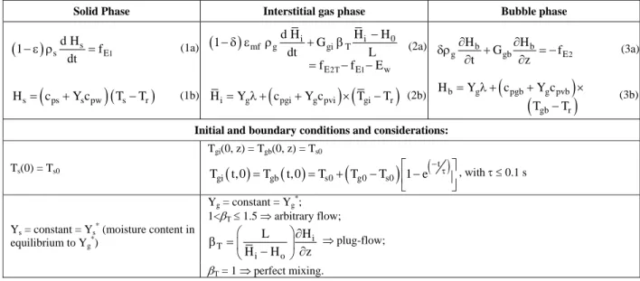
The Vitor et al. heat transfer model (Vitor et al., 2004) assumes that the solid phase is perfectly mixed, while the bubble phase is moving upwards through the bed in plug-flow. The interstitial gas phase can flow in the perfect mixing or in an arbitrary flow regime between the plug-flow and the perfect mixing. Another assumption is that this gas phase is the one responsible for losing energy to ambient air through the column wall. Table 1 summarizes the energy balance equations of the model.
Table 2 schematizes the interactions between these three phases. Note that this model is a simplified version of the drying model under the condition of no water evaporation, meaning that the solid moisture content and the gas humidity are in equilibrium.
Table 1: Energy balance equations from Vitor et al. model (Vitor et al., 2004).
Solid Phase Interstitial gas phase Bubble phase
( )
1s
s E
d H
1 f
dt
− ε ρ = (1a)
( )
2T 1
i i 0
mf g gi T
E E w
d H H H
1 G
dt L
f f E
−
− δ ε ρ + β
= − −
(2a)
2
b b
g gb E
H H
G f
t z
∂ ∂
δρ + = −
∂ ∂ (3a)
(
)
(
)
s ps s pw s r
H = c +Y c T −T (1b) Hi= λ +Yg
(
cpgi+Y cg pvi) (
× Tgi−Tr)
(2b)(
)
(
)
b g pgb g pvb gb r
H Y c Y c
T T
= λ + + ×
− (3b)
Initial and boundary conditions and considerations:
Ts(0) = Ts0
Tgi(0, z) = Tgb(0, z) = Ts0
( )
( )
(
)
( )
tgi gb s0 g0 s0
T t,0 =T t,0 =T + T −T ⎡⎢1 e− −τ ⎤⎥
⎣ ⎦, with τ≤ 0.1 s
Yg = constant = Yg*; 1<βT≤ 1.5 ⇒ arbitrary flow;
i T
i o
L H
H H z
⎛ ⎞ ∂
β = ⎜ − ⎟ ∂
⎝ ⎠ ⇒ plug-flow;
Ys = constant = Ys* (moisture content in equilibrium to Yg*)
Brazilian Journal of Chemical Engineering Vol. 26, No. 03, pp. 545 - 554, July - September, 2009
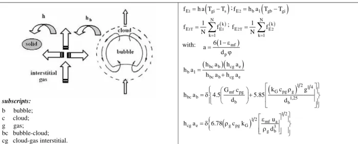
Table 2: Interactions between phases (after Vitor et al., 2004)
(
)
1
E gi s
f =h a T −T ;fE2=h ab 1
(
Tgb−Tgi)
( )
1T 1
N k
E E
k 1
1
f f
N =
=
∑
; ( )2T 2
N k
E E
k 1
1
f f
N =
=
∑
with: ( mf)
p
6 1 a
d
− ε
= ϕ
( bc b)
(
cg e)
b 1
bc b cg e
h a h a
h a
h a h a
= +
(
)
1 2 1 4 G pg g mf pgbc b 1,25
b b
k c g
G c
h a 4.5 5.85
d d
⎫
⎡ ρ ⎤
⎧ ⎛ ⎞
⎪ ⎢ ⎥⎪
= δ⎨ ⎜ ⎟+ ⎢ ⎥⎬
⎪ ⎝ ⎠
⎩ ⎣ ⎦⎭⎪
subscripts: b bubble; c cloud; g gas;
bc bubble-cloud; cg cloud-gas interstitial.
(
)
{
1 21 2 mf a
cg e g pg G 3
g b
u
h a 6.78 c k
d
⎫ ⎡ε ⎤ ⎪
= δ ρ ⎢ρ ⎥ ⎬
⎢ ⎥ ⎪
⎣ ⎦ ⎭
The rate of heat loss through the column wall is expressed as:
(
)
(
)
L L
bed
w W amb wa w amb
bed bed
A A
E T T T T
V V
= α − = α − (4)
where αW is the overall heat transfer coefficient that
combines the bed-wall (αbw) coefficient, the
wall-ambient (αwa) coefficient and the wall thermal
resistance; AL = π Dc L is the lateral area of the bed
column; Vbed = π Dc2 L/4 is the bed volume;Tbed is the mean gas temperature along the bed height, obtained by the enthalpy balance for the bubble and interstitial gas mixture;Tw is the mean column wall temperature along the bed height and Tamb is the
room ambient air temperature. Victor et al. (2004) has used αW as the model parameter to calculate Ew.
The heat transfer coefficient between gas interstitial and bubble (hb) is determined using the
correlations proposed by Kunii and Levenspiel (1969). As discussed later, these correlations are specific for each Geldart group of particles. The heat transfer coefficient between particle and interstitial gas, h, are expressed as a function of Rep:
(
2)
gi x
1 p p
k
h x Re
d
= (5)
Therefore, four adjustable model parameters (1 ≤βT
≤ 1.5; αW or αwa; x1 and x2) must be estimated using
experimental data together with the model solution.
Victor et al. (2004) have obtained these parameters for tapioca (Geldart group B particle) in a cylindrical column of Dc = 0.102 m; Lmf = 0.101 m and Dc/dp =
185. The DASSL computational code (Petzold, 1989) is used to solve the model differential-algebraic system of equations (see Table 1) after discretization of the z spatial coordinate. The parameter estimation procedure comprises two methods: the heuristic one of PSO optimization (Kennedy and Eberhart, 1995) to locate the rough solution and the maximum likelihood method of ESTIMA computational code (Noronha et al., 1991) to refine the rough solution.
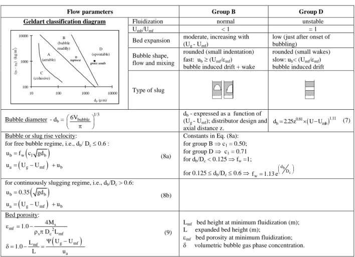
However, as one can see in Table 3, gas flows quite differently in fluidized beds of group D particles than in fluidized beds of group B particles. Therefore, for describing heat transfer mechanisms in fluidized beds of Geldart group D particles, the Vitor et al. model, as well as its computational solution procedure, must be modified to conform to the fluid flow behavior in these types of beds.
Moreover, according to the two-phase theory, the gas flow is divided between the bubble phase and the dense phase as:
(
)
(
)
gb g mf g g mf
G = Ψ G −G = ρ Ψ U −U (6)
Modified Model
Equations (7), (8a) and (8b) and their restrictions (see Table 3) are incorporated into the model for better describing the gas flow in fluidized beds of group D particles. In the computational program developed for solving the modified model, the wall effect on the bubble rise velocity is taken as the model restriction even when db/Dc > 0.125.
Moreover, the axial distance z, at which the transition between bubbling and slugging regimes occurs, is determined previously (taking db = 0.6 Dc
in Eq. (7)) in order to establish the flow regime along the bed height. This information is fundamental to estimate the volumetric bubble concentration (δ) and the volumetric heat transfer coefficient between cloud and interstitial gas (hcgae), which depend on
the mean bubble or slug velocity, as one can see in Tables 2 and 3. Note that, in the laboratory scale fluidized bed unit, wall effects and changes in the fluid flow regime can strongly affect the heat transfer mechanisms.
To uncouple Ew from the gas temperature, the
wall heat transfer coefficient, αwa (presented in Eq.
(4)), is chosen as the one adjustable parameter of this modified model. Therefore, the mean column wall temperature should be measured during the experiments. It is important to mention that, in the fluidized bed design, this wall temperature can be fitted by choosing the appropriate material to build the column.
Although optimization methods used in this work are those proposed by Vitor et al. (2004), the number of adjustable parameters has been reduced to three (αwa; x1 and x2) by setting values of βT, i.e.:
βT = 1 ⇒ gas interstitial phase in perfect mixing; βT = 1.5 ⇒ gas interstitial phase in arbitrary flow; and
i
T
i o
L H
H H z
⎛ ⎞ ∂
β = ⎜ − ⎟ ∂
⎝ ⎠ ⇒
gas interstitial phase in
plug-flow.
Table 3: Flow regime for particles from Geldart group B and D (Geldart, 1986)
Flow parameters Group B Group D
Fluidization normal unstable
Umb/Umf < 1 = 1
Bed expansion moderate, increasing with (Ug - Umf)
low (just after onset of bubbling)
Bubble shape, flow and mixing
rounded (small indentation) fast: ub≥ (Umf/εmf) bubble induced drift + wake
rounded (small wakes) slow: ub< (Umf/εmf) bubble induced drift Geldart classification diagram
100 1000 10000
10 100 1000 10000 dp (μm)
(≅
s
- ≅
g
)
(k
g
/m
3)
A (aerable)
B (bubble readilly)
C (cohesive)
D (spoutable)
grass seads tapioca
Type of slug
Bubble diameter - db =
1/3 bubble
6V
⎛ ⎞
⎜ π ⎟
⎝ ⎠
db - expressed as a function of (Ug - Umf); distributor design and
axial distance z. ( )
1.11 0.81
b mb
d =2.25z × −U U (7)
Constants in Eq. (8a): for group B ⇒ c1 = 0.50;
for group D ⇒ c1 = 0.71 Bubble or slug rise velocity:
for free bubble regime, i.e., db/ Dc≤ 0.6 :
(
)
(
)
b w 1 b
a g mf b
u f c gd
u U U u
=
= − +
(8a) for d
b/Dc < 0.125 ⇒ fw =1; for 0.125 ≤ db/Dc≤ 0.6 ⇒
b c d
D w
f 1.13 e
⎛ ⎞
⎜ ⎟
⎝ ⎠
=
for continuously slugging regime, i.e., db/Dc > 0.6:
( )
(
)
b b
a g mf b
u 0.35 gd
u U U u
=
= − +
(8b)
Bed porosity:
(
)
s
mf 2
s c mf g mf mf
a
4M 1.0
D L
U U
L 1.0
L u
ε = − ρ π
Ψ −
δ = − =
(9)
Lmf bed height at minimum fluidization (m); L expanded bed height (m);
εmf bed porosity at minimum fluidization;
Brazilian Journal of Chemical Engineering Vol. 26, No. 03, pp. 545 - 554, July - September, 2009
MATERIALS AND METHODS
Particle Characterization
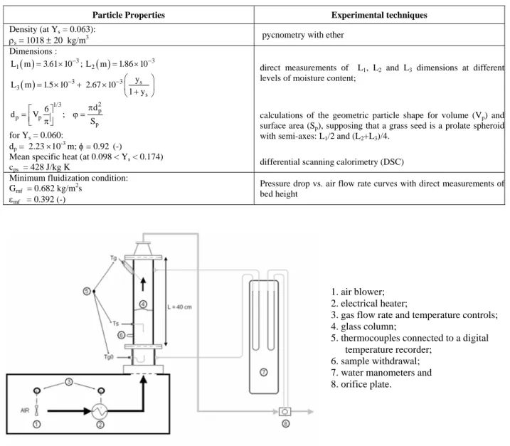
The physical properties of Brachiaria brizantha grass seeds used in the experiments are shown in Table 4. As already corroborated in Table 3, these seeds belong to the Geldart group D.
Experimental Setup
The experimental setup is shown in Figure 1. The laboratory scale fluidized bed column, built in glass
to allow the visualization of the fluidized bed regime, is 0.07 m in diameter and 0.40 m in height. Air is drawn by a centrifugal fan, inserted into a closed cabinet at the bottom of the column. This air passes through a mesh filter, a 2 kW electrical heater and a mesh plate distributor, before fluidizing the bed of particles. Leaving the column, exit air passes through a calibrated orifice plate for recording the air flow rate, which is controlled by a valve located inside the cabinet. As shown in Figure 1, a water manometer is used to measure the actual pressure drop across the bed.
Table 4: Properties of the grass seeds and experimental techniques employed
Particle Properties Experimental techniques
Density (at Ys = 0.063):
ρs = 1018 ± 20 kg/m3
pycnometry with ether Dimensions :
( ) 3 3( )
1 2
L m =3.61 10× − ; L m =1.86 10× −
( ) 3 3 s
3
s
y
L m 1.5 10 2.67 10
1 y
− − ⎛ ⎞
= × + × ⎜ + ⎟
⎝ ⎠
direct measurements of L1, L2 and L3 dimensions at different levels of moisture content;
2 1/3
p
p p
p
d 6
d V ;
S
π ⎡ ⎤
=⎢ ⎥ ϕ = π
⎣ ⎦
for Ys = 0.060:
dp = 2.23 ×10⁻³ m; φ = 0.92 (-)
calculations of the geometric particle shape for volume (Vp) and surface area (Sp), supposing that a grass seed is a prolate spheroid with semi-axes: L1/2 and (L2+L3)/4.
Mean specific heat (at 0.098 < Ys < 0.174) cps = 428 J/kg K
differential scanning calorimetry (DSC) Minimum fluidization condition:
Gmf = 0.682 kg/m2s
εmf = 0.392 (-)
Pressure drop vs. air flow rate curves with direct measurements of bed height
1. air blower; 2. electrical heater;
3. gas flow rate and temperature controls; 4. glass column;
5. thermocouples connected to a digital temperature recorder;
6. sample withdrawal; 7. water manometers and 8. orifice plate.
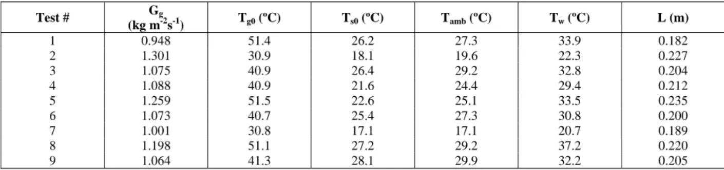
Table 5: Operational conditions of experiments
Test # Gg
(kg m-2s-1) Tg0 (ºC) Ts0 (ºC) Tamb (ºC) Tw (ºC) L (m)
1 0.948 51.4 26.2 27.3 33.9 0.182 2 1.301 30.9 18.1 19.6 22.3 0.227 3 1.075 40.9 26.4 29.2 32.8 0.204 4 1.088 40.9 21.6 24.4 29.4 0.212 5 1.259 51.5 22.6 25.1 33.5 0.235 6 1.073 40.7 25.4 27.3 30.8 0.200 7 1.001 30.8 17.1 17.1 20.7 0.189 8 1.198 51.1 27.2 29.2 37.2 0.220 9 1.064 41.3 28.1 29.9 32.2 0.205
Three copper-constantan thermocouples are installed inside the column to measure: the inlet air temperature, Tg0, (thermocouple inserted just before
the distributor plate); the solid-gas emulsion temperature, Tbed, or the solid temperature, Ts,
(thermocouple placed 0.10 m above the air distributor) and the outlet air temperature, TgL,
(thermocouple placed at z = 0.38 m from the base of the column). The solid temperature, Ts, is measured
during a short time interval in which the bed is collapsed; details of this method are discussed by Rizzi Jr. et al. (2005). A thermocouple adhered to the outer column wall (at z =0.38 m) records the column wall temperature, Tw. Another thermocouple, located
close to the experimental unit, registers the ambient temperature for each experiment. A laboratory humidity indicator measures the inlet air humidity.
Experimental Procedure
Heat transfer experiments are performed following the factorial design in two levels of the inlet air temperature, Tg0, and air flow rate, Gg ,
using three replications at the central point, as shown in Table 5 (test #1 to #7). Further experiments, tests # 8 and #9, are also carried out in the laboratory unit to validate the modified model. In all tests, the mass of grass seeds is set at 0.350 kg with the average moisture Ys = 0.06 = Ys* at the inlet air humidity of
Yg = 0.012 and the range of the inlet air temperature
given in Table 5. Replications (experiments #3, #4 and #6) are used to evaluate the data reproducibility and the experimental errors.
RESULTS AND DISCUSSION
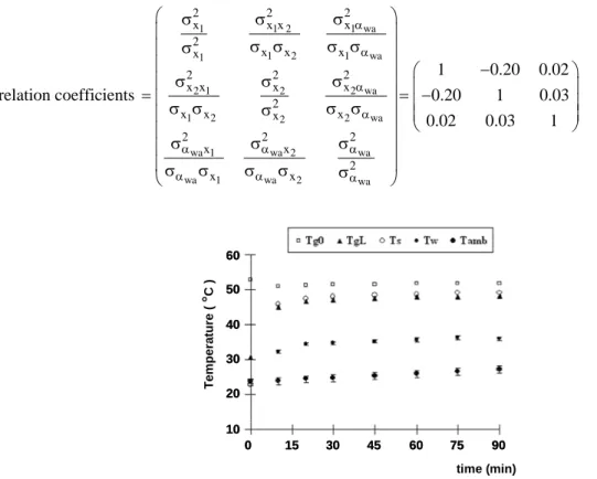
A typical data set obtained from experiments is shown in Figure 2. The maximum experimental error is ± 1ºC from measurements of Tamb at the central
point replications. The experimental error for the other measured temperatures is equal to (or less than)
± 0.5 ºC. Trends observed in Figure 2 are expected. For the processing time greater than 60 min., the solid temperature, Ts, equals to the gas outlet
temperature, TgL. The wall temperature, Tw, tends to
increase until reaching its equilibrium value at 60 min. At this time, TgL approaches to the inlet air
temperature, Tg0, but TgL does not match to Tg0
because heat is lost through the column wall.
Although the wall temperature (Tw) depends on
the processing time and on the axial distance z, its value, used in Eq. (4), is equal to the time-average from measurements obtained at z = 0.38 m. Time-oscillations in the ambient temperature (Tamb) and in
the inlet gas temperature (Tg0) are punctually
neglected. Their values, used in the model solution, are time-averages of their measurements during each experiment.
Following the same procedure proposed by Vitor et al. (2004), in which the PSO and ESTIMA optimization codes are incorporated to the DASSL model solution program, data obtained from tests #1 to #7 are used to estimate x1, x2 and αwa for each
supposed value of βT, i.e., βT =1 (gas interstitial in
perfect mixing); βT = 1.5 (gas interstitial in arbitrary
flow) and i
T
i o
L H
H H z
⎛ ⎞ ∂
β = ⎜ − ⎟ ∂
⎝ ⎠ (gas interstitial in
plug-flow).
The best results are obtained when the gas interstitial is in the plug-flow regime. Table 6 presents these results for Ψ = 1. The matrix of the correlation coefficients, shown in Eq. (10), indicates little correlation between these parameter, i.e., between x1 and x2, x1 and αwa and x2 and αwa. Note
that if two parameters are uncorrelated or independent, their correlation coefficient tends to be zero. If this coefficient approaches to 0.9, there is a strong correlation between the two parameters. In addition, a negative value of this coefficient means that large values of one variable are associated with small values of the other (in this case: x2 with x1 and
Brazilian Journal of Chemical Engineering Vol. 26, No. 03, pp. 545 - 554, July - September, 2009
correlation coefficients
1 wa
1 1 2
1 2 1 wa
1
2 wa
2 1 2
1 2 2 2 wa
wa 1 wa 2 wa
wa 1 wa 2 wa
2
2 2
x
x x x
2
x x x
x
2
2 2
x
x x x
2
x x x x
2 2 2
x x
2
x x
1 0.20 0.02
0.20 1 0.03
0.02 0.03 1
α α
α α
α α α
α α α
⎛ σ σ σ ⎞
⎜ ⎟
σ σ σ σ
σ ⎜ ⎟ ⎜ ⎟ ⎛ − ⎞ σ σ σ ⎜ ⎟ ⎜ ⎟
=⎜ σ σ σ σ ⎟ ⎜= − ⎟
σ ⎜ ⎟
⎜ ⎟ ⎝ ⎠
⎜ σ σ σ ⎟
⎜ ⎟
⎜σ σ σ σ σ ⎟
⎝ ⎠ (10) Te m p e ra tu re ( ° C )
0 15 30 45 60 75 90
60 50 40 30 20 10 time (min) Te m p e ra tu re ( ° C )
0 15 30 45 60 75 90
0 15 30 45 60 75 90
0 15 30 45 60 75 90
60 50 40 30 20 10 60 50 40 30 20 10 time (min)
Figure 2: Typical experimental data (test # 5 in Table 5).
Table 6: Best values of adjustable model parameters for the gas interstitial in plug-flow regime
Model parameters x1 (-)* x2 (-)* αwa (W/K m2)**
Estimation value 4.11×10⁻² 1.55×10⁻¹ 2.75×101
Standard deviation (σ) 1×10⁻⁴ 5×10⁻⁴ 3×10⁻¹
(*) see Eq. (5); (**) see Eq. (4).
Little correlation between these model parameters and their low standard deviation attest to a good statistical estimation of these parameters from experimental data. From the theoretical point of view, Figure 3 shows that the slugging regime is supposed to exist in almost the entire bed (slugs arrive at z/L ≤ 0.3). This justifies the choice of Ψ = 1
and explains the best results for the plug-flow of the gas interstitial phase.
By using the values of the adjustable parameters given in Table 6 under conditions of plug-flow for the gas interstitial phase and Ψ = 1, tests #8 and 9 have been simulated by the model. In Figure 4, experimental data are compared to those simulated by the model.
0.0 0.2 0.4 0.6 0.8 1.0
0 0.02 0.04 0.08 0.06 db (m ) z/H SLUG
0.0 0.2 0.4 0.6 0.8 1.0
0.0 0.2 0.4 0.6 0.8 1.0
0 0.02 0.04 0.08 0.06 0 0.02 0.04 0.08 0.06 db (m ) z/H SLUG
0.0 0.2 0.4 0.6 0.8 1.0
0 0.2 0.4 0.6 bubl e veloci ty (m /s) z/H SLUG
0.0 0.2 0.4 0.6 0.8 1.0
0.0 0.2 0.4 0.6 0.8 1.0
0 0.2 0.4 0.6 0 0.2 0.4 0.6 bubl e veloci ty (m /s) z/H SLUG (a) (b)
50 40 30 20 10 0
0 15 30 45 60 75 90
time (min) T - simulated
Te m p e ra tu re ( ° C )
T - exp. T - simulated
T - exp. s gL gL s 50 40 30 20 10 0
0 15 30 45 60 75 90
time (min) T - simulated
Te m p e ra tu re ( ° C )
T - exp. T - simulated
T - exp. 50 40 30 20 10 0
0 15 30 45 60 75 90
time (min) T - simulated
Te m p e ra tu re ( ° C )
T - exp. T - simulated
T - exp. s gL gL s 50 40 30 20 10 0
0 15 30 45 60 75 90
time (min) T - simulateds
Te m p e ra tu re ( ° C )
T - exp.s T - simulatedgL
T - exp.gL 50 40 30 20 10 0
0 15 30 45 60 75 90
time (min) T - simulateds
Te m p e ra tu re ( ° C )
T - exp.s T - simulatedgL
T - exp.gL
(a) (b) Figure 4: Comparison between experimental and simulated data: (a) test #8; (b) test #9.
From Figure 4, one can see the good agreement between experimental and simulated data, basically at t > 15 minutes. Although there is no experimental measurement in the first transient period (0 ≤ t ≤ 15 minutes) for comparison, the simulated outlet air temperature seems to increase abruptly during the first seconds (from TgL0 = Ts0 = Tamb to TgL at 1
minute). Such an abrupt unexpected increase in the simulated TgL must be related to the wall
temperature, which is taken as a constant in the model solution. Based on experimental data (see Figure 2), Tw also depends on time, increasing in the
transient period until reaching its constant value. Another assumption that needs to be verified is the Ψ value. Although Geldart (1986) and Rhodes (1990) have suggested Ψ = 1 for the slugging regime, flow conditions obtained in fluidized beds of seeds are transitional between bubbling and slugging regimes (see Figure 3), inducing a progressive change in Ψ from 0.26 (Geldart group D particles) to 1.
Besides all these controversies, the heat transfer model predicts quite well the experimental data for the range of parameters used in this work.
CONCLUSION
The three-phase model proposed by Victor et al. (2004) has been well modified to describe the heat transfer mechanisms in fluidized beds of particles belonging to Geldart group D (in the present case: seeds of Brachiaria brizantha) and to uncouple one of the wall heat transfer coefficients from the outlet gas temperature. Results show good agreement
between experimental and simulated data, obtained from the modified model.
As the first step for simulating the drying of
Brachiaria brizantha in fluidized beds, this work also discusses flow regimes of the interstitial and bubble gas phases and their implications in determining the heat transfer coefficients between these phases. Studies are in progress to extend these results for the drying operation.
NOMENCLATURE
AL lateral area of the bed
column = π DcL,
m2 a specific exchange
superficial area between gas and particles,
m-1
cp specific heat J kg-1 K-1
c1 parameter dependent on
particle size, specified in Table 3
(-)
Dc column diameter m
d diameter m
Ew rate of energy loss through
column wall per unit of bed volume
J s-1 fw wall effect factor defined in
Table 3
(-)
G air mass flow rate per cross sectional area of the column
kg m-2 s-1
H specific enthalpy m2 s-2
h effective heat transfer
coefficient between solids and interstitial gas phase
Brazilian Journal of Chemical Engineering Vol. 26, No. 03, pp. 545 - 554, July - September, 2009
hbcab volumetric heat transfer
coefficient between bubble and cloud
J m-3 s-1 K-1
hcgae volumetric heat transfer
coefficient between cloud and interstitial gas
J m-3 s-1 K-1
hba1 volumetric heat transfer
coefficient between bubble and interstitial gas phase
J m-3 s-1 K-1
Hcol height of the column m
kg thermal conductivity of gas kg s
-3
L expanded bed height m
T temperature ºC or K
t time s
U superficial gas velocity m/s
ub rise velocity of an isolated
bubble or slug
m/s
ua mean bubble or slug
velocity
m/s
V volume m3
VB bed volume = π Dc2 L/4 m
3
x1, x2 parameters in Equation 5
Y water content in dry basis (-)
Y* equilibrium moisture content
(-)
z axial coordinate m
Greek Symbols
αw heat transfer coefficient
between column walls and air ambient
J s-1 m-2 K-1
β coefficient related with the interstitial gas phase
(-)
δ volumetric bubble concentration
(-)
ε bed porosity (-)
φ particle sphericity (-)
λ latent heat of vaporization J kg-1
μ viscosity kg s-1 m-1
ρ density kg m-3
Ψ ratio of the visible bubble flow to the excess gas velocity
(-)
Special Subscripts
0 initial value amb ambient bed bed b bubble
exp experimental g gas
gL exit gas
i interstitial gas l liquid water m gas-solid mixture mb minimum bubbling
condition
mf minimum fluidization condition
out outlet p particle s solid v water vapor w wall
Dimensionless Numbers
Nu Nusselt number = h.dp/kgi
Rep Reynolds number of particle = Ggi.dp/μgi
ACKNOWLEDGMENTS
The authors would like to thank CAPES for the Ph.D. scholarship of A.C. Rizzi Jr. and Dr. J. F. A. Vitor for the free copies of the computer programs.
REFERENCES
Geldart, D., Gas Fluidization Technology. John Willey & Sons Inc., New York, NY (1986). Groenewold, H., Tsotsas, E., A New Model for Fluid
Bed Drying, Drying Technology, 15 (6-8), 1687 (1997).
Hilligardt, K., Werther, J., Local Bubble Gas Hold-up and Expansion of Gas/Solid Fluidized Beds, Germ.Chem.Eng., 9, 215 (1986).
Kunii, D., Levenspiel, O., Fluidization Engineering. John Willey & Sons Inc., New York, NY (1969). Noronha, F. B., Pinto, J. C., Monteiro, J. L., Lobão, M. W., Santos, T. J., ESTIMA: Um Pacote Computacional para Estimação de Parâmetros e Projeto de Experimentos, Technical Report, PEQ/COPPE/UFRJ, Rio de Janeiro, Brazil (in Portuguese) (1993).
Rhodes, M. J., Principles of Powder Technology, John Wiley & Sons Ltd., New York, NY (1990). Rizzi Jr., A. C., Passos, M. L., Freire, J. T., Drying
of Grass Seeds (Brachiaria brizantha) in fluidized bed. Part I: Preliminary Studies, (in portuguese), In Proceedings of the XXXI Brazilian Congress of Particulate Systems (XXXI ENEMP 2004), Uberlândia-MG, CD-ROM (2005).
Vitor, J. F. A., Biscaia Jr., E. C. and Massarani, G.,
Modeling of Biomass Drying in Fluidized Bed, In Proceedings of the 14th International Drying Symposium (IDS 2004), São Paulo-SP, CD-ROM (1104-1111) (2004).
Wildhagen, G. R. S., Calçada, L. A., Massarani, G., Drying of porous Particles in Fluidized Beds: Modeling and Experiments, Journal of Porous Media, 2(5), 123 (2002).