Algorithms
ASHFAQUE AHMED MEMON*, NAEEM AZIZ MEMON*, AND KAMRAN ANSARI*
RECEIVED ON 08.02.2012 ACCEPTED ON 21.06.2012
ABSTRACT
An effort has been made to optimally determine the status of turbulence loss coefficient in the present study. The parameter is identified in the framework of GA (Genetic Algorithm), which consequently resulted in the development of a computer model. In accordance with principles of the GA, the objective function, sse (sum of square of errors), is minimized between 0.009785 and 0.017565; as a result the well hydraulic parameters are optimally identified. To check validity of the model, simulated draw downs are compared against the observed ones, which indicate mean difference between them varying from 0.0049m to 0.0124m. Furthermore, validity of the model is also endorsed through statistical analysis with model efficiency varying between 99.97 and 100.00%. The model is applied to 5 data sets of step drawdown pumping test, yielding 5 values of turbulence coefficient varying between 1.01 and 2.08. Out of these 5 optimized values of turbulence coefficient none of the values is equal to 2. This scenario of variation of turbulence coefficient substantiate that turbulence coefficient is a variable and not a constant (i.e. equal to 2.0, as suggested by Jacob and Singh) while considering turbulence loss coefficient as a constant is discarded.
Key Words: Turbulence Loss Coefficient, Well Hydraulic Parameters, Optimization, Genetic Algorithm.
*Assistant Professor, Department of Civil Engineering, Mehran University of Engineering & Technology, Jamshoro.
1.
INTRODUCTION
status of last parameter i.e. turbulence loss coefficient. Some of the researchers opine that it has a constant value of 2.0, whereas others suggest it as a variable. At the preliminary stage, when Jacob [1] established the relationship for drawdown or loss of head in a pumping well under steady-state; he suggested that turbulence loss coefficient (n) have a constant value of 2. Rorabaugh [2] proposed turbulence loss coefficient as variable between 2.4 and 2.8 for higher discharges. Moreover, he categorized n for various flow conditions and termed this
Determination of Turbulence Coefficient using Genetic Algorithms
loss as; laminar loss for low discharges with n=1.0; and turbulent loss in case of high discharges with n>2.0. Lennox [3] considered turbulence loss coefficient as variable and proposed its upper limit equal to 3.5. According to Sheahan, [4] turbulence loss coefficient may have a value between 1 and 4. Todd [5] opines that exact value of n cannot be fixed since it varies from well to well depending upon internal and external flow conditions of the well. Whereas, Singh [6] agreed with the constant value of 2 for turbulence loss coefficient as suggested by Jacob's, [1]. But, recently Louwyck, et. al. [7] termed n as well loss power and considered it as a variable with lower limit of 1.0. Traditionally, aquifer parameters have been identified by analyzing the step-drawdown test using a graphical method suggested by Jacob, [1]. However, this method is subjective in nature, time-consuming, prone to error and possesses intrinsic limitations.
With availability of high-speed computers and evolution of different numerical techniques, graphical solution can be efficiently replaced by some suitable numerical solution in the form of a computer model. A number of conventional optimization techniques such as Marquardt algorithm, Dynamic programming, Guass-Newton method and Gradient projection are available in literature, which by virtue of their inherited characteristic yield local optima. On the other hand, counterparts of the former ones are the unconventional optimization techniques, which merit in achieving global optima. Such techniques include GAs (Genetic Algorithms), GP (Genetic Programming), SA (Simulated Annealing), SCE (Shuffled Complex Evolution) method developed at the UA (University of Arizona) and ANN (Artificial Neural Network). Savic, et. al. [8-9] determined optimal location of isolating valves using GA, Khu, et. al. [10] applied GP for forecasting real-time runoff, Savic, et al. [11] developed a rainfall-runoff model using GP, Duan, et. al. [12] used SCE-UA optimization technique for calibration
of watershed models, Rogers, et. al. [13] developed solute transport and groundwater remediation model using ANN, Simpson, et. al. [14] used GA for pipe optimization, Ejaz et, et. al. [15] automized weight selection for robust controller design using GA and Ranjithan, et. al. [16] applied ANN for groundwater reclamation. Moreno, et. al. [17] optimized groundwater pumping, by connecting various variables related to hydrology, topography, and economics, etc., using MATLAB. Their analysis reveals that steepness of the characteristic curve, pumping pipe diameter and maximum efficiency depends on the fluctuation of the groundwater table, water demand and month of highest demand, respectively.
Determination of Turbulence Coefficient using Genetic Algorithms
For the past few years GA has been widely used by hydrologists and hydro-geologists for solution of groundwater and solute transport problems. Memon, et. al. [21] used GA as an optimization tool for identification of aquifer parameters. Cieniawski, et. al. [22] employed GA to solve multi-objective groundwater monitoring problem. Gwo, [23] tried to search flow paths in structured porous media by use of GA. McKinney, et. al. [24] gave GA solution of groundwater management models. Parsad, et. al. [25] while estimating net aquifer recharge and conductivity zones, they used GA. Reed, et. al. [26] designed a groundwater monitoring plan on long term basis while using GA. Ritzel, et. al. [27] solved a multi-objective solute transport problem using GA. In this research work GA technique is employed to optimally identify the turbulence loss coefficient, which ultimately resulted in development of a computer model coded in C++ language.
In this paper after brief description of the GA technique, problem of estimating the optimal value of well hydraulic parameters (including turbulence loss coefficient) is formulated to be solved in the framework of genetic algorithm, so that subjective graphical solution can be avoided. Boundary conditions to be incorporated in the GA model for the three well parameters are set. Also, setting of string length, genetic parameters, population size and number of generations for the code is described. Finally, simulated results are compared with the field observations and sensitivity analysis of the model is carried out.
2.
GENETIC ALGORITHM
The GA is an evolutionary computing technique developed by research group of John, [28] at the University of Michigan. They tried to develop a robust tool, in accordance with biological processes of survival and adaptation that could be capable of maintaining balance between efficiency and efficacy necessary for survival in many different environments (Holland, [28]
and Goldberg, [29]). With continuous contribution by various researchers, at present GAs have become highly idealized and multidimensional search algorithms based on the concepts of natural selection and natural genetics. Due to their robustness and some other characteristics, GAs are being extensively used as an optimization tool in the fields of science, commerce, and engineering.
Coding for GAs can be done either by using real or binary values of the parameters, later being more powerful and dependable in search of optimal values (Goldberg, et. al. [30]). Since, in the present work binary coded genetic algorithm is used, therefore, forthcoming discussion is related to the features related to these types of GAs. Computational procedure for search and optimization of any problem by GAs must include following five basic steps (Michalewicz, [31]), viz: (1) Representation, in which binary vectors or strings are used to represent real values of the independent variables involved in the system to be solved; (2) Initial Population, i.e. a number of chromosomes are generated such that each chromosome is a binary vector of bits (genes); (3) Evaluation function, includes evaluation and rating of potential solutions contained in population of chromosomes by putting real values of binary vectors into the function; (4) Genetic operators (crossover and mutation), used for reproduction i.e. alteration of the present population to form new population; and (5) Genetic Parameters (probability of crossover and probability of mutation), define the extent of alteration by the genetic operators
3.
PROBLEM FORMULATION
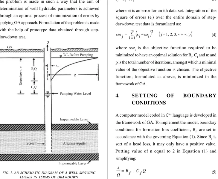
A well penetrating throughout the depth of an aquifer is subjected to formation and well losses. Formation loss is domino effect of the aquifer properties, whereas well loss is on account of friction met due to radially inward motion of water to the well and of its uptake towards the pumping device (Fig. 1). According to Jacob, [1], formation loss is the product of Bf and Q, and the well loss of Cf and Qn,
Determination of Turbulence Coefficient using Genetic Algorithms
where Q is the pumping discharge of the well. Hence, the total drawdown for a well running at discharge (Q) under steady state condition is:
s = BfQ + CfQn (1)
From equation (1) it can be seen that for a given discharge, Q, s is the function of Bf, Cf and n parameters. Proper estimation of s requires prior knowledge of these parameters; thus, the objective of the present research is aimed at to optimally determine the above mentioned well hydraulic parameters with special attention to value of n.
In order to achieve the desired objective, formulation of the problem is made in such a way that the aim of determination of well hydraulic parameters is achieved through an optimal process of minimization of errors by applying GA approach. Formulation of the problem is made with the help of prototype data obtained through step-drawdown test.
In equation (1), if an observed value of Q is introduced; and also if Bf, Cf and n values are incorporated by selecting them randomly within the range of their given boundary conditions, then for an ith data-set a drawdown (si) could be computed as:
n i Q f C i Q f B i
s = + (2)
Where, i = 1, 2, 3, ……., m; and m is the total number of data-sets. Residue of the difference between simulated drawdown (si) and observed drawdown (soi) ushers into an error computed as:
e
i = si - soi (3)
where ei is an error for an ith data-set. Integration of the square of errors (ei) over the entire domain of step-drawdown test data is formulated as:
(
)
(
j 1,2,3, ,p)
m 1 i
2 i so i s j
sse ∑ = LL
= −
= (4)
where ssej is the objective function required to be minimized to have an optimal solution for Bf, Cf and n; and p is the total number of iterations, amongst which a minimal value of the objective function is chosen. The objective function, formulated as above, is minimized in the framework of GA.
4.
SETTING OF BOUNDARY
CONDITIONS
A computer model coded in C++ language is developed in
the framework of GA. To implement the model, boundary conditions for formation loss coefficient, Bf, are set in accordance with the governing Equation (1). Since Bf is sort of a head loss, it may only have a positive value. Putting value of n equal to 2 in Equation (1) and simplifying:
Q f C f B Q
s
+
= (5)
Q
Accordingly, it can be construed from Equation (5) that while 'CfQ' tends to 's/Q' then Bf reaches to 0, which characterizes its lower boundary, and when 'CfQ' attains to 0 then Bf tends towards 's/Q', which marks its upper boundary condition. Therefore, the boundary conditions for Bf are set as 0 and 3.0. Boundary conditions for entry loss coefficient, Cf, are set in accordance with suggestions made by Walton, [32]. According to him Cf depends upon well condition; Table 1 contains such information and hence in line with his suggestions the boundary conditions for Cf are set as 0 and 5.0. Jacob, [1] and Singh, [6] suggested a constant value of 2 for turbulence loss coefficient, n, whereas Rorabaugh [2], Lennox [3], Sheahan [4], Todd's [5] and Louwyck, et. al. [7] argued that n may have different value than 2.0. Consequently, the boundary conditions for n are set at 1.0 and 4.0.
5.
RUNNING OF GA MODEL
For determination of the well hydraulic parameters and investigation of the status of turbulence loss coefficient, the computer model developed in the framework of GA prerequisites discharge-drawdown data for its execution. For this purpose the model was applied to 5 (published and unpublished) data-sets of step-drawdown test.
In line with the boundary conditions set for execution of the model a precision of 2 digits after decimal point was fixed for Bf and Cf, whereas a precision of 3 digits after decimal point was fixed for n. Based on these characteristics chromosome lengths of 9, 9 and 12 binary digits were required for Bf, Cf and n, respectively. Hence, total length of a chromosome became 30 binary digits.
The computer model was run for numerous iterations to obtain a minimized value of the objective function, sse. To achieve the objective of minimization of sse, the model
parameters; such as POPSIZE (Population Size), Pc (probability of crossover) and Pm (probability of mutation) were fixed through trial and error and are obtained as 110, 0.85 and 0.015, respectively. Trial and error approach was adopted since change in these parameters influence the diversity level within the chromosomes which in turn affect the optimal values of the unknown parameters i.e. Bf, Cf and n, and eventually the objective function, sse. POPSIZE is set to vary from 10~170 by an increment of 10 and with each POPSIZE, the NOGEN (Number of Generations) is allowed to vary in between 100 and 3000 with a constant step size of 100, and under these conditions for each iteration minimized value of the objective function, sse is recorded.
6.
RESULTS DISCUSSION
6.1
GA Model Application and Results
The optimal values of the well hydraulic parameters were obtained for the minimal objective function varying between 0.009785 and 0.21054; Table 2 shows these optimal values. From Table 2 the optimal values of turbulence loss coefficient are plotted as shown in Fig. 2. These values of turbulence loss coefficient vary between 1.01 and 2.80.
TABLE 1. ENTRY LOSS COEFFICIENT (Cf) FOR VARIOUS CONDITIONS OF WELL [32]
Properly designed and well developed <0.5
Mildly deteriorated or clogged 0.5-1.0
Severely deteriorated or clogged 1.0-4.0
Difficult to restore to its original condition >4.0
TABLE 2. WELL HYDRAULIC PARAMETERS FOR 5 DATA-SETS OF STEP-DRAWDOWN PUMPING TEST
Data Set Bf Cf n
1 0.28 0.01 2.80
2 0.10 0.22 1.32
3 0.29 0.03 1.59
4 0.41 0.02 1.80
5 0.39 0.05 1.01
Determination of Turbulence Coefficient using Genetic Algorithms
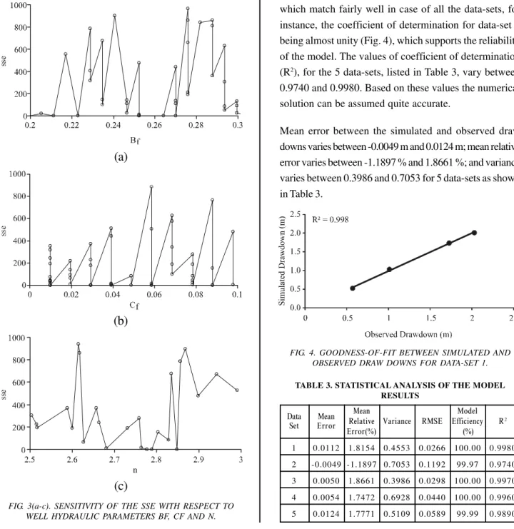
Sensitivity of the model is measured in terms of minimization of the objective function, sse, with respect to well hydraulic parameters Bf, Cf and n. Fig. 3(a-c) show plotting segments for a data-set. The figures exhibit jumbled phenomena with numerous spikes allowing identifying optimal values for the well hydraulic parameters while the objective function is realized at least minimal level.
6.2
Validity of the Model
Validity of the model was tested using simulated and observed values to ensure model applicability. If results of comparison between the observed and simulated values indicate good agreement, then the model can be recommended.
Simulated values were compared with the observed ones which match fairly well in case of all the data-sets, for instance, the coefficient of determination for data-set 1 being almost unity (Fig. 4), which supports the reliability of the model. The values of coefficient of determination (R2), for the 5 data-sets, listed in Table 3, vary between
0.9740 and 0.9980. Based on these values the numerical solution can be assumed quite accurate.
Mean error between the simulated and observed draw downs varies between -0.0049 m and 0.0124 m; mean relative error varies between -1.1897 % and 1.8661 %; and variance varies between 0.3986 and 0.7053 for 5 data-sets as shown in Table 3.
FIG. 3(a-c). SENSITIVITY OF THE SSE WITH RESPECT TO WELL HYDRAULIC PARAMETERS BF, CF AND N.
TABLE 3. STATISTICAL ANALYSIS OF THE MODEL RESULTS
Data Mean Mean Model
Set Error Relative Variance RMSE Efficiency R2
Error(%) (%)
1 0.0112 1.8154 0.4553 0.0266 100.00 0.9980
2 -0.0049 -1.1897 0.7053 0.1192 99.97 0.9740
3 0.0050 1.8661 0.3986 0.0298 100.00 0.9970
4 0.0054 1.7472 0.6928 0.0440 100.00 0.9960
5 0.0124 1.7771 0.5109 0.0589 99.99 0.9890
(a)
(b)
(c)
Validity and performance of the model was also checked statistically by computing RMSE (Root Mean Square error) and model efficiency (EF) as shown in Table 3. These parameters indicate the goodness-of-fit between measured and simulated values; their variation is 0.0266~0.1192m and 99.97~100.00%, respectively. Based on these results it can be concluded that the model is dependable and can be a useful tool to apply in practice.
7.
CONCLUSION
In the present study, effort has been made to develop a computer model in the framework of GA for determination of optimal values of well hydraulic parameters with special attention to turbulence loss coefficient. In accordance with the principles of GA, the objective function, sse is minimized and varies as 0.009785~0.21054; correspondingly the well hydraulic parameters Bf, Cf and n are optimally identified. Validity of the model was also tested by plotting simulated draw downs against the observed ones; the gradient of line obtained for each data-set being almost unity, hence the numerical solution is assumed to be quite accurate. Mean difference between the simulated and observed draw downs, mean relative error and variance varied as -0.0049~0.0124, -1.1897~0.8661%, and 0.3986~0.7053, respectively. The statistical parameters, RMSE and EF were computed and varied from 0.0266-0.1192m and from 99.97-100.00%, respectively. These parameters indicate the high goodness-of-fit between measured and simulated values. Based on these results it can be concluded that the model is dependable and can be applied in practice. The optimal values of turbulence loss coefficient (n) vary between 1.01 and 2.80; hence, assumption of Jacob [1] and Singh [6] for it as a constant value is discarded; conversely opinion of Rorabaugh [2], Lennox [3], Sheahan [4], Todd's [5] and Louwyck, et. al. [7] for considering it as a variable is ascertained.
ACKNOWLEDGEMENTS
Authors are very much grateful to HEC (Higher Education Commission), Pakistan, Islamabad, for sponsoring this research. Authors would also like to express their sincere gratitude to Mehran University of Engineering & Technology, Jamshoro, Pakistan, for allowing them to carry out that research work.
REFERENCES
[1] Jacob, C.E., "Drawdown Test to Determine Effective Radius of Artesian Well", Transactions of ASCE, Volume 112, pp. 1047-1070, USA, 1947.
[2] Rorabaugh, M.I., "Graphical and Theoretical Analysis of Step-Drawdown Test of Artesian Well”, Proceedings of Hydraulic Division, ASCE, Volume 79, pp. 362-384, USA, 1953.
[3] Lennox, D.H., "Analysis and Application of Step-Drawdown Tests", Journal of Hydraulic Division, ASCE, 92, Volume 6, pp. 25-47, USA, 1966.
[4] Sheahan, N.T., "Type-curve solution of step-drawdown test", Groundwater, 9(1), 25-29, USA, 1971.
[5] Todd, D.K., "Groundwater Hydrology", John Wiley and Sons, 2nd Edition, pp. 152-153, Singapore, 1995.
[6] Singh, S.K., "Well Loss Estimation: Variable Pumping Replacing Step-Drawdown Test", Journal of Hydraulic Engineering, ASCE, Volume 128, No. 3, pp. 343-348, USA, 2002.
[7] Louwyck, A., Vandenbohede, A., and Lebbe, L., "Numerical Analysis of Step-Drawdown Test: Parameter Identification and Uncertainty", Journal of Hydrology, Volume 380, pp. 165-179, Elsiver, 2010.
[8] Savic, D.A., and Walters, G.A., "An Evolution Program for Optimal Pressure Regulation in Water Distribution Networks", Engineering Optimization, Volume 24, No. 3, pp. 197-219, UK, 1995.
[9] Savic, D.A., and Walters, G.A., "Integration of a Model for Hydraulic Analysis of Water Distribution Networks with an Evolution Program for Pressure Regulation", Micro Computing in Civil Engineering, ASCE, Volume 10, No. 3, pp. 219-229, USA, 1995b.
Determination of Turbulence Coefficient using Genetic Algorithms
[11] Savic, D.A., Walters, G.A., and Davidson, J.W., "A Genetic Programming Approach to Rainfall Runoff Modeling",
Water Resources Management, Volume 13, pp. 219-231, Springer, 1999.
[12] Duan, Q., Sorooshian, S., and Gupta, V.K., "Optimal Use of the SCE-UA Global Optimization Method for
Calibrating Watershed Models", Journal of Hydrology,
Volume 158, pp. 265-284, Elsivier, 1994.
[13] Rogers, L.L., and Dowla, F.U., "Optimization of
Groundwater Remediation Using Artificial Neural Networks with Parallel Solute Transport Modeling",
Water Resources Research, Volume 30, No. 2, pp. 457-481, USA, 1994.
[14] Simpson, A.R., Dandy, G.C., and Murphy, L.J., "Genetic Algorithms Compared to Other Techniques for Pipe
Optimization", Journal of Water Resources Planning
and Management, ASCE, Volume 120, No. 4, pp. 423-443, 1994.
[15] Ejaz, M., Arbab, M.N., and Khan, L., "Automatic Weight Selection in H∞ Shaping Using GA", Mehran University
Research Journal of Engineering and Technology, Volume 26, No. 2, pp. 179-190, Jamshoro, Pakistan, April, 2007.
[16] Ranjithan, S., and Eheart, J.W., "Neural Network-Based Screening for Groundwater Reclamation Under
Uncertainty", Water Resources Research, Volume 29,
No. 3, pp. 563-574, USA, 1993.
[17] Moreno, M.A., Córcoles, J.I., Moraleda, D.A., Martinez,
A., and Tarjuelo, J.M., "Optimization of Underground Water Pumping", Journal of Irrigation and Drainage
Engineering, ASCE, Volume 136, No. 6, USA, 2010.
[18] Majumdar, P.K., Mishra, G.C., Sekhar, M., and Sridharan,
K., "Coupled Solution for Forced Recharge in Confined Aquifers", Journal of Hydrologic Engineering, ASEC,
Volume 14, No. 12, USA, 2009.
[19] Onwunalu, J.E., and Durlofsky, L.J., "Application of a
Particle Swarm Optimization Algorithm for Determining
Optimum Well Location and Type", Computer Geosciences, Volume 14, pp. 183-198, Springer, 2010.
[20] Ciaurri, D.E., Isebor, O.J., and Durlofsky, L.J., "Application of Derivative-Free Methodologies to
Generally Constrained Oil Production Optimisation Problems", International Journal of Mathematical
Modelling and Numerical Optimisation,Volume 2, No.
2, pp. 134-161, USA, 2011.
[21] Memon, A.A., Babar, M.M., and Kori, S.M., "Identification of Aquifer Parameters Using Genetic Algorithm", Mehran University Research Journal of Engineering & Technology, Volume 26, No. 2, pp. 97-110, Jamshoro, Pakistan, April, 2007.
[22] Cieniawski, S.E., Eheart, J.W., and Ranjithan, S., "Using Genetic Algorithms to Solve a Multiobjective Groundwater Monitoring Problem", Water Resources Research, Volume 31, No. 2, pp. 399-409, USA, 1995.
[23] Gwo, J.P., "In Search of Preferential Flow Paths in Structured Porous Media Using a Simple Genetic Algorithm", Water Resources Research, Volume 37, No. 6, pp. 1589-1601, USA, 2001.
[24] McKinney, D.C., and Lin, M.D., "Genetic Algorithm Solution of Groundwater Management Models", Water Resources Research, Volume 30, No. 6, pp. 1897-1906, USA, 1994.
[25] Prasad, K.L., and Rastogi, A.K., "Estimating Net Aquifer Recharge and Zonal Hydraulic Conductivity Values for Mahi Right Bank Canal Project Area, India by Genetic Algorithm", Journal of Hydrology, Volume 24, No. 3, pp. 149-161, Elsivier, 2001.
[26] Reed, P., Minisker, B.S., and Valocchi, A.J., "Cost-Effective Long-Term Groundwater Monitoring Design Using a Genetic Algorithm and Global Mass Interpolation", Water Resources Research, Volume 36, No. 12, pp. 3731-3741, USA, 2000.
[27] Ritzel, B.J., and Eheart, W., "Using Genetic Algorithms to Solve a Multiple Objective Groundwater Pollution Containment Problem", Water Resources Research, Volume 30, No. 5, pp. 1589-1603, USA, 1994.
[28] Holland, J.H., "Adaptation in Natural and Artificial Systems", MIT Press, 2nd Edition, Cambridge, Massachusetts, USA, 1992.
[29] Goldberg, D.E., "Genetic Algorithms in Search, Optimization and Machine Learning", Addison-Wesley Publishing Company Inc., New York, USA, 1989.
[30] Goldberg, D.E., Korb, B., and Deb, K., "Messy Genetic Algorithms: Motivation, Analysis and First Results", Complex Systems, Volume 3, No. 5, pp. 493-530, USA, 1989.
[31] Michalewicz, Z., "Genetic Algorithms + Data Structures = Evolution Programs", 3rd Edition Revised and Extended, Springer Verlag, Berlin, Germany, 1999.