TOPOGRAFIA E VARIABILIDADE ESPACIAL DE PROPRIEDADES FÍSICAS DO SOLO

(1)

TOPOGRAPHY AND SPATIAL VARIABILITY OF

SOIL PHYSICAL PROPERTIES

Marcos Bacis Ceddia1_{*; Sidney Rosa Vieira}2_{; André Luis Oliveira Villela}3_{; Lenilson dos}

Santos Mota5_{; Lúcia Helena Cunha dos Anjos}1_{; Daniel Fonseca de Carvalho}4

1

UFRRJ - Depto. de Solos, BR 465 - km 7 - 23900-000 - Seropédica, RJ - Brasil. 2

IAC - Centro de Solos e Recursos Ambientais, C.P. 28 - 13020-902 - Campinas, SP - Brasil. 3

UFRRJ - Programa de Pós-Graduação em Agronomia-Ciência do Solo. 4

UFRRJ - Depto. de Engenharia - BR 465 - km 7 - 23900-000 - Seropédica, RJ - Brasil. 5

UFRRJ - Graduando em Engenharia Agronômica. *Corresponding author <ceddia@ufrrj.br>

ABSTRACT: Among the soil formation factors, relief is one of the most used in soil mapping, because of its strong correlation with the spatial variability of soil attributes over a landscape. In this study the relationship between topography and the spatial variability of some soil physical properties was evaluated. The study site, a pasture with 2.84 ha, is located near Seropédica, Rio de Janeiro State, Brazil, where a regular square grid with 20 m spacing was laid out and georreferenced. In each sampling point, altitude was measured and undisturbed soil samples were collected, at 0.0– 0.1, 0.1–0.2, and 0.2–0.3 m depths. Organic carbon content, soil texture, bulk density, particle density, and soil water retention at 10 (Field Capacity), 80 (limit of tensiometer reading) and 1500 kPa (Permanent Wilting Point) were determined. Descriptive statistics was used to evaluate central tendency and dispersion parameters of the data. Semivariograms and cross semivariograms were calculated to evaluate the spatial variability of elevation and soil physical attributes, as well as, the relation between elevation and soil physical attributes. Except for silt fraction content (at the three depths), bulk density (at 0.2–0.3 m) and particle density (at 0.0–0.1 m depth), all soil attributes showed a strong spatial dependence. Areas with higher elevation presented higher values of clay content, as well as soil water retention at 10, 80 and 1500 kPa. The correlation between altitude and soil physical attributes decreased as soil depth increased. The cross semivariograms demonstrated the viability in using altitude as an auxiliary variable to improve the interpolation of sand and clay contents at the depth of 0.0–0.3 m, and of water retention at 10, 80 and 1500 kPa at the depth of 0.0–0.2 m.

Key words: terrain elevation, geostatistics, soil physics, cross semivariance

TOPOGRAFIA E VARIABILIDADE ESPACIAL DE

PROPRIEDADES FÍSICAS DO SOLO

RESUMO: O relevo é um dos fatores de formação do solo mais usados em mapeamento de solos devido sua forte correlação com a variabilidade espacial de atributos do solo na paisagem. O objetivo desse trabalho foi avaliar a relação entre topografia e a variabilidade espacial de algumas propriedades físicas de solos. Em uma pastagem com 2,84 ha instalou-se uma grade regular com espaçamento de 20 m, nas proximidades de Seropédica, RJ, onde cada ponto de amostragem foi georreferenciado. Em cada ponto de amostragem foi medida a altitude e foram coletadas amostras indeformadas nas profundidades de 0,0–0,1; 0,1–0,2 e 0,2–0,3 m. Determinaram-se os teores de carbono, textura, densidade do solo e das partículas e retenção de água a 10, 80 e 1500 kPa. Estatística descritiva foi usada para avaliar a tendência central e a dispersão dos dados. Semivariogramas simples e cruzados foram usados para avaliar a variabilidade espacial da altitude, e dos atributos físicos do solo, bem como a relação entre altitude e atributos físicos do solo. Com exceção da fração silte (nas três profundidades), densidade do solo (0,2–0,3 m) e densidade das partículas (0,0–0,1 m), todos os atributos apresentaram forte dependência espacial. Encontraram-se maiores teores de argila, bem como de retenção de água a 10, 80 e 1500 kPa, nas cotas mais elevadas. A correlação entre altitude e atributos físicos decresceu com o aumento da profundidade. Os semivariogramas cruzados comprovaram a viabilidade do uso da altitude, por cokrigagem, para aperfeiçoar a interpolação de areia e argila na camada de 0.0–0.3 m, e de retenção de água a 10, 80 e 1500 kPa na camada de 0.0–0.2 m.

(2)

INTRODUCTION

Soil sampling allows the characterization of several soil attributes which may be estimated at unsampled sites through existing models. Determinis-tic models are considered to be more appropriate when there is enough information on physical and chemical properties, and allow the understanding of the phenom-enon as a whole (Isaaks & Srivastava, 1989). How-ever, very few processes are understood enough to al-low the use of such models.

The use of deterministic models for the un-derstanding of both soil formation and their attributes does not result in accurate estimation, because of the great complexity among soil properties (Webster, 2000). Probabilistic models admit some uncertainty about how the phenomenon succeeds, and available data are considered as results of a random process (Isaaks & Srivastava, 1989). The geostatistics focus is based on a probabilistic model, and has been suc-cessfully used in soil science for a quantitative de-scription of spatial variability, which may support pre-dictions about the phenomena investigated (Vieira, 2000).

The identification of landscape features is an important tool used by pedologists in their soils map-ping procedures. The use of landscape elevation digi-tal models has increased predictions on soil parameters from terrain attributes. Since topography parameters, defined from primary and secondary attributes, con-trols water and sediments distribution over the scape, researchers have been trying to correlate land-scape features (altitude, slope, shape) with physical soil attributes (Kreznor et al., 1989; Pachepsky et al., 2001; Sobieraj et al., 2002; Rezaei & Gilkes, 2005). Spatial variability of soil color and texture were considered feasible to be used in models of digital soil mapping in Southern of Amazon (Novaes Filho et al., 2007). Many authors also evidenced the influences of landforms on soil physical properties. Working with soils of northeastearn of Sao Paulo State, Souza et al. (2004) found that small variations in the landscape form de-fined different spatial variability in soil physical at-tributes. Similar results were found by Souza et al. (2003), which evaluate the effect of landforms on anisotropy of soil physical attributes and observed higher spatial variability of soil physical attributes in the concave landform when compared to the linear one. Considering the importance of mapping spa-tial variability of soil physical attributes and its rela-tion with relief, the objective of this study was to evaluate the relationship between topography and the spatial variability of some soil physical properties in a hillside area used as a pasture.

MATERIAL AND METHODS

Semivariograms

The experimental semivariogram, γ(h), of n spatial observations z(x_i), i = 1, ... n, can be calcu-lated using

( )

_{( )}

N( )h

[

( ) (

)

]

2

1 i

i

i Z x h

x Z h N 2 1 h

∑

= + − =

γ (1)

where N(h) is the number of observations separated by a distance h. Experimental semivariograms can be fit in to a variety of models that have well known pa-rameters: nugget C₀, sill (C₀+ C₁), and range of spa-tial dependence (a), McBratney & Webster (1986). Equation (1) is obtained from a derivation starting at the intrinsic hypothesis, under which there is no re-quirement for existence of a finite variance of the ob-servations, Var (z). Only stationarity of the differences [(Z(x_i) – Z(x_i+ h)] are required for its derivation (Journel & Huijbregts, 1978).

Scaled semivariograms

The scaling technique of semivariograms was developed by Vieira et al. (1997) and expressed as:

( )

i i sc i h h α γ =

γ i = 1,2,…,m (2)

where γsc(h) is the scaled semivariogram, γ(h) the original semivariogram, α

i is the scale factor and m

is the number of measured variables. The scale fac-tor α is a constant that can take the value of the cal-culated variance - the sill when it exists - or the high-est value of the semivariogram γ(h). The idea is that if semivariograms of properties sampled over the same field scale together on the same graph then their spatial variabilities can be related to common causes.

Cross-semivariogram

It is possible that spatial dependence between two variables exists and it may be used in the estima-tion of one of them using both of them using cokriging. Vauclin et al. (1983) used cokriging and observed that there was a decrease in the cokriging estimation vari-ances as compared to the kriging. Spatial dependence between two variables Z₁ and Z₂ can be expressed by the cross semivariogram

)] x ( Z -h) + x ( Z )][ x ( Z -h) + x ( Z [ 2N(h) 1 =

(h) 1 1i 1 1i 2 2j 2 2j

N(h) 1 = i 12

∑

γ (3)

(3)

variable changes in the opposite direction as the other. Cokriging development can be found elsewhere (Goovaerts, 1997; Vieira, 2000).

Study site and sampling procedures

The study site has 2.84 ha and is located be-tween 43°40’ and 43°41’ W, and 22°44’ and 22°45’ S, in the Seropédica municipality, Rio de Janeiro State, Southeastern region of Brazil. The area has pasture coverage implanted in 1997 and was formed exclu-sively by the Transvala grass (Digitaria decumbens

Stent cv Transvala).

In order to apply geostatistics to investigate the spatial variability of soil physical attributes, the sam-pling strategy included the definition of a 20 m spac-ing square grid. Since spacspac-ing between samplspac-ing points might affect data modeling, additional soil samples were collected in a reduced spacing (1, 5 and 10 m), according to topography and soil classes, as recom-mended by Trangmar et al. (1985). In each of the 89 sampling points, altitude and UTM coordinates were measured using a GPS with differential correction (DGPS - Trimble-GeoExplorer 3 model), with submetric accuracy.

Soil chemical and physical analysis

Undisturbed soil samples were collected at depths of 0.0–0.1, 0.1–0.2 and 0.2–0.3 m, for the de-termination of water retention at 10 (field capacity), 80 (limit of a tensiometer reading), 1,500 kPa (per-manent wilting point) and soil bulk density - ρ_b (double-cylinder method) (Embrapa, 1997). Readily available water capacity (EAWC = 10 kPa – 80 kPa) and avail-able water capacity (AWC = 10 kPa – 1,500 kPa) in-dices were calculated from the water retention data. Loose soil samples were grinded and air-dried for de-termination of: soil particle density - ρ_s (volume de-termination method), soil particle size distribution (Pi-pette method) (Embrapa, 1997) and organic carbon content (Walkley & Black, 1934).

Statistical analysis

Descriptive and exploratory analysis was performed to find both the central tendency and dispersion of data. BioEstat 2.0 (Ayres et al., 2003) and XLSTAT 7.5 (Addinsoft, 2004) softwares were used to evaluate the existence of outliers, as well as to perform both normality and Pearson correlation tests. Geostat (Vieira et al., 1983) soft-ware was used both to determine measures of spa-tial continuity (experimental semivariograms) and for model fitting to the semivariogram to be further used in the interpolation. The selection of the most proper model was done by cross-validation (jack knifing).

RESULTS AND DISCUSSION

Descriptive analysis

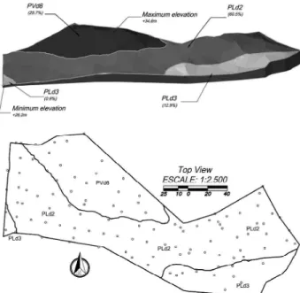
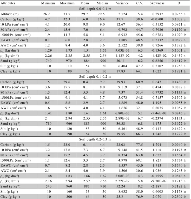
The descriptive statistical results for altitude and soil physical attributes are in Table 1. Samples were col-lected along a slope, with altitude values ranging from 26.2 to 33.7 meters above the sea level. The soil map unities (Figure 1) identified in the area were: PVD6 -Loamy over fine clayey Kandiudult; PLD2 -Paleudult; and PLD3 - association of Paleudults + Aquents (Soil Survey Staff, 1999). ThePaleudults with sandy over loamy texture were more common (74.3%), and were preferentially found on the mid-slope and on the foot

slope. Loamy over fine clayey Kandiudult were the

dominant soil class on the hill tops (25.7%).

Due to the greater occurrence of sandy over loamy Paleudults, and the sampling restricted to the upper 0.3 m, the dominant class of texture at the three sampled depths was sandy, and it greatly influenced the other soil attributes, resulting in low water reten-tion and availability. The sandy texture also influenced the bulk density values, which were considered to be relatively high (averaging 1.51–1.61 kg dm–3

), as well as soil particle density for the three depths (averaging 2.55–2.57 kg dm–3

). Those soil particle density values result from the dominance of the quartz mineral in the sand fraction (Silva et al., 2001).

The contents of sand, silt and clay were found to be quite similar at the 0.0–0.1 m, and 0.1–0.2 m depths. At the 0.2–0.3 m depth data showed a greater variance, despite the average value being very similar

(4)

to the upper depths. This may result from the fact that the 0.2–0.3 m layer is coincident to the upper bound-ary of a transitional zone to an argillic horizon (B) in the Ultisols. The small effect of this greater variance within the mean values of sand, silt and clay contents is explained by the small occurrence of sampling points with high clay contents.

The water retention capacity at 10, 80 and 1,500 kPa, and the available water capacity (EAWC

and AWC) decreased with increasing soil depth, which can be explained by the reduction of organic carbon content and a small increase in the clay content up to the 0.3 m depth, a common characteristic of the up-per layers of the soils studied, especially the Paleudults (Planossolos, according to EMPRAPA, 2006), the most common soil class in the study site.

Analyzing the statistical parameters (Table 1) it is possible to evaluate the frequency distribution of

Attributes Minimum Maximum Mean Median Variance C.V. Skewness D

Soil depth 0.0-0.1 m

Altitude (m) 26.2 33.5 29.7 29.5 2.524 5.4 0.2937 0.0755 n

Carbon (g kg–1₎ _4.7 _32.3 _16.0 _16.4 _37.7 _38.6 _-0.0500 _{0.1002 n}

10 kPa (cm3_cm–3₎ _4.1 _20.0 _9.8 _9.0 _12.67 _36.4 _0.5152 _{0.0921 n}

80 kPa (cm3_cm–3₎ _2.4 _15.6 _7.0 _6.4 _9.792 _44.7 _0.7936 _{0.1179 ln}

1500kPa (cm3_cm–3₎ _1.9 _11.7 _5.8 _5.1 _6.932 _45.6 _0.6783 _{0.1070 ln}

EAWC (cm3_cm–3₎ _0.1 _6.0 _2.8 _2.7 _1.805 _48.5 _0.2132 _{0.0822 n}

AWC (cm3_cm–3₎ _1.2 _8.4 _4.0 _3.6 _2.522 _39.8 _0.7266 _{0.1392 ln}

r_b (kg dm–3₎ _1.29 _1.73 _1.51 _1.53 _9.03E-03 _6.3 _-0.1369 _{0.1001 n}

r_s (kg dm–3₎ _2.26 _2.85 _2.55 _2.56 _1.13E-02 _4.2 _{-1.42E-02 0.1457 n}

Sand (g kg–1₎ ₇₄₀ ₉₇₀ ₈₈₄ ₉₀₀ _30.11 _6.2 _-0.8256 _{0.1617 ln}

Silt (g kg–1₎ ₁₀ ₁₁₀ ₅₄ ₅₀ _6.404 _47.2 _0.2102 _{0.1258 n}

Clay (g kg–1₎ ₁₀ ₁₈₀ ₆₂ ₅₀ _17.83 _64.1 _1.022 _{0.1821 ln}

Carbon (g kg–1₎ _1.5 _29.6 _10.4 _9.7 _39.93 _60.9 _0.643 _{0.1430 ln}

10 kPa (cm3_cm–3₎ _3.6 _15.5 _8.1 _8.0 _9.119 _37.1 _0.4741 _{0.0882 n}

80 kPa (cm3_cm–3₎ _1.5 _12.4 _5.3 _4.8 _7.37 _51.4 _0.7732 _{0.1135 ln}

1500kPa (cm3_cm–3₎ _0.8 _9.1 _4.1 _3.7 _5.073 _54.8 _0.7157 _{0.1507 ln}

EAWC (cm3_cm–3₎ _0.5 _8.8 _2.9 _2.7 _1.889 _48.0 _1.195 _{0.0985 ln}

AWC (cm3_cm–3₎ _1.6 _9.2 _4.0 _4.1 _1.676 _32.1 _0.8075 _{0.1057 ln}

r_b (kg dm–3₎ _1.41 _1.80 _1.61 _1.61 _6.80E-03 _5.1 _{-5.46E-02 0.0846 n}

r_s (kg dm–3₎ ₂ _2.94 _2.55 _2.56 _2.89E-02 _6.7 _-0.2374 _{0.1153 n}

Sand (g kg–1₎ ₇₁₀ ₉₆₀ ₈₈₃ ₉₀₀ _36.38 _6.8 _-1.175 _{0.1922 ln}

Silt (g kg–1₎ ₁₀ ₁₂₀ ₅₃ ₅₀ _6.361 _48.9 _0.447 _{0.1622 n}

Clay (g kg–1₎ ₁₀ ₁₉₀ ₆₄ ₅₀ _19.55 _66.3 _1.248 _{0.1772 ln}

Carbon (g kg–1₎ _1.5 _23.0 _6.1 _4.4 _22.03 _77.5 _1.794 _{0.0940 ln}

10 kPa (cm3_cm–3₎ _3.2 _17.6 _7.3 _6.7 _9.148 _41.5 _1.114 _{0.1193 ln}

80 kPa (cm3_cm–3₎ _1.4 _15.2 _4.5 _3.7 _8.374 _63.8 _1.622 _{0.1554 ln}

1500kPa (cm3_cm–3₎ _1.1 _12.6 _3.3 _2.7 _4.978 _68.1 _1.825 _{0.1774 ln}

EAWC (cm3_cm–3₎ _0.7 _8.2 _2.8 _2.5 _1.537 _45.0 _1.713 _{0.1540 ln}

AWC (cm3_cm–3₎ _2.1 _8.4 _4.0 _3.9 _1.506 _30.6 _1.036 _{0.1263 ln}

r_b (kg dm–3₎ _1.48 _1.83 _1.66 _1.67 _5.08E-03 _4.3 _-0.1555 _{0.0846 n}

r_s (kg dm–3₎ _2.16 _2.94 _2.57 _2.56 _2.22E-02 _5.8 _{-9.70E-02 0.1213 n}

Sand (g kg–1₎ ₅₄₀ ₉₆₀ ₈₈₁ ₉₁₀ _52.24 _8.2 _-2.187 _{0.2182 ln}

Silt (g kg–1₎ ₁₀ ₁₆₀ ₅₃ ₅₀ _8.632 _58.0 _0.9003 _{0.1178 ln}

Clay (g kg–1₎ ₁₀ ₃₀₀ ₆₆ ₅₀ _25.8 _76.9 _2.079 _{0.2509 ln} D – Maximum dispersion in relation to normal distribution; n – Normally distributed at a confidence interval >0.95; Ln – Log normally distributed at a confidence interval >0.95 (Kolmogorov-Smirnov statistic test).

(5)

the variables. Skewness values up to 0.5 suggest a spe-cific attribute with normal distribution (Webster, 2001). Besides altimetry, the only attributes that showed both features, skewness smaller than 0.5 and normal dis-tribution, at the three depths, were soil bulk density and particle density. Moreover, skewness values tended to increase with increasing soil depth, as well as the maximum errors of the frequency distribution tests (D values). This behavior can be evidenced by the at-tributes 10 kPa, EAWC, and silt, for which the fre-quency distribution is normal at the upper depths and becomes lognormal as depth increases.

The smallest CV values (> 10%) were found for altitude, soil bulk density, particle density, and sand fraction content, at the three depths. The other at-tributes showed relatively high values (> 30%). The clay fraction had the highest CV values, and the CV for water retention increased proportionally to the wa-ter tension force. The high values of CV for clay con-tent can be explained by the great amplitude of varia-tion in the area (minimum e maximum values, Table 1), as well as, higher error associated to clay suction in the pipette method. In general, CV values increased with increasing soil depth, except for EAWC, AWC and soil bulk density. Variance and CV had a similar pat-tern for particle density, sand, silt, and clay fraction

contents, and increased with depth. On the other hand, variance and CV for organic carbon content, water re-tention at field capacity, at 80 kPa, and at permanent wilting point decreased with increasing in depth.

Similar performance for water retention data was found by Mallants et al. (1996), observing the vari-ance tendency to decrease with increasing depth, as the CV increases. Water release through more uniform pores may explain it, particularly for high water ten-sion values. In this study, lower variance for high wa-ter tension values may be explained by wawa-ter reten-tion caused by adsorpreten-tion rather than capillarity (as at 10 and 80 kPa), which is more erratic, since it is strongly controlled by porosity.

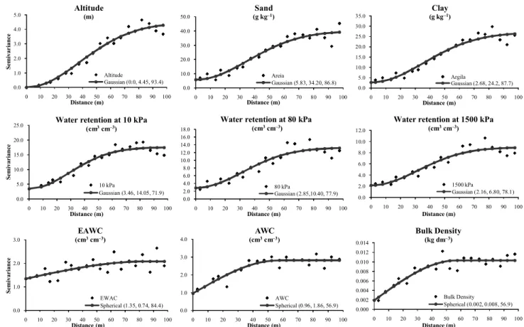
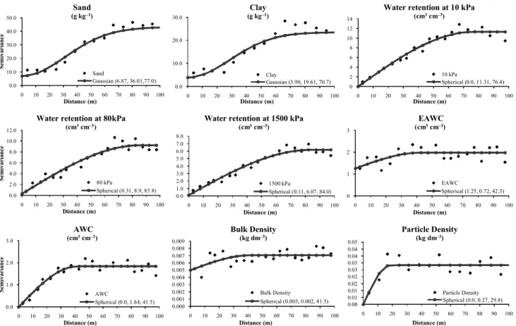
Evaluation of semivariograms

Experimental semivariograms, fitted models and respective parameters at each depth are presented in Table 2, and Figures 2, 3 and 4, respectively. Two types of semivariograms were observed, according to the variable and the soil depth. The first type, pure nug-get effect, was observed for the silt fraction content (at the three depths) and particle density (0.0–0.1 m). The pure nugget effect indicates the absence of spa-tial correlation. This suggests that, for those variables at their respective depths, the mean, the median or the

Figure 2 - Experimental and fitted theoretical semivariograms for altitude and the soil attributes at 0.0–0.1 m depth.

0.0 2.0 4.0 6.0 8.0 10.0 12.0 14.0 16.0 18.0

0 10 20 30 40 50 60 70 80 90 100

Distance (m)

Water retention at 80 kPa

(cm3_cm–3₎

80 kPa

Gaussian (2.85,10.40, 77.9) 0.0 5.0 10.0 15.0 20.0 25.0

0 10 20 30 40 50 60 70 80 90 100

Semivariance

Distance (m)

(cm3_cm–3₎

10 kPa

Gaussian (3.46, 14.05, 71.9) 0.0 10.0 20.0 30.0 40.0 50.0

0 10 20 30 40 50 60 70 80 90 100

Distance (m)

Sand

(g kg–1₎

Areia

Gaussian (5.83, 34.20, 86.8) 0.0 5.0 10.0 15.0 20.0 25.0 30.0 35.0

0 10 20 30 40 50 60 70 80 90 100

Distance (m)

Clay

(g kg–1₎

Argila

Gaussian (2.68, 24.2, 87.7)

0.0 2.0 4.0 6.0 8.0 10.0 12.0

0 10 20 30 40 50 60 70 80 90 100

Distance (m)

(cm3_cm–3₎

1500 kPa

Gaussian (2.16, 6.80, 78.1)

0.0 1.0 2.0 3.0

0 10 20 30 40 50 60 70 80 90 100

Semivariance

Distance (m)

EAWC

(cm3_cm–3₎

EWAC

Spherical (1.35, 0.74, 84.4) 0.0 1.0 2.0 3.0 4.0

0 10 20 30 40 50 60 70 80 90 100

Distance (m)

AWC

(cm3_cm–3₎

AWC

Spherical (0.96, 1.86, 56.9) 0.000 0.002 0.004 0.006 0.008 0.010 0.012 0.014

0 10 20 30 40 50 60 70 80 90 100

Distance (m)

Bulk Density

(kg dm–3₎

Bulk Density

Spherical (0.002, 0.008, 56.9) 0.0 1.0 2.0 3.0 4.0 5.0

0 10 20 30 40 50 60 70 80 90 100

Semivariance

Distance (m)

Altitude

(m)

Altitude

(6)

mode may be the best estimator in any point of the studied area, if distribution is normal (Journel & Huijbregts, 1978).

In the second type, increasing distance (h) re-sulted in an increased γ(h), up to a maximum stable value. The distance at which γ(h) reaches stability is called range (a), and it is defined as the limit distance of spatial dependence (Vieira, 2000). Altitude, sand and clay fractions, water retention at 10, 80 and 1,500 kPa, EAWC, AWC, soil bulk density and particle density (at the depth 0.2–0.3 m), presented this type of

semivariogram. This in agreement to the intrinsic hy-pothesis, and may be considered that the stationary of order 2.

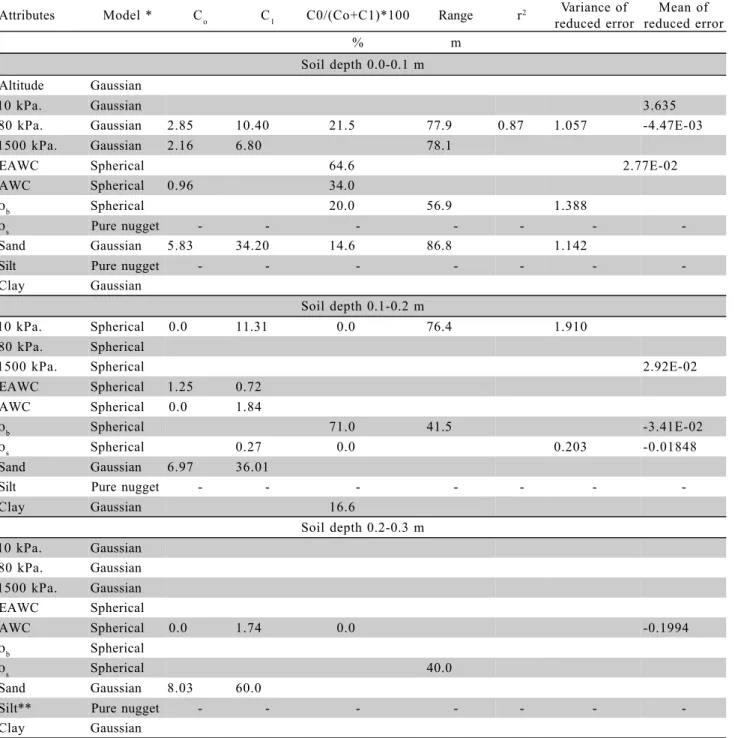
Altitude, sand and clay contents (at the three depths) fitted a Gaussian model, but soil bulk density, particle density (except at 0–0.10 m depth), EAWC and AWC showed a pattern of spherical model at the three depths. Some attributes showed patterns matching dif-ferent models with soil depth, as water retention ca-pacity at 10, 80 and 1500 kPa. In this case, the Gaussian model fitted at depths 0.0–0.10 m and 0.20– Table 2 - Parameter values for the estimated theoretical semivariogram.

*Models fitted according to Jack-nife procedure. **After removal of the linear trend.

Attributes Model * C_o C₁ C0/(Co+C1)*100 Range r2 Variance of

reduced error

Mean of reduced error

% m

Soil depth 0.0-0.1 m Altitude Gaussian

10 kPa. Gaussian 3.635

80 kPa. Gaussian 2.85 10.40 21.5 77.9 0.87 1.057 -4.47E-03

1500 kPa. Gaussian 2.16 6.80 78.1

EAWC Spherical 64.6 2.77E-02

AWC Spherical 0.96 34.0

r_b Spherical 20.0 56.9 1.388

r_s Pure nugget - - -

-Sand Gaussian 5.83 34.20 14.6 86.8 1.142

Silt Pure nugget - - -

-Clay Gaussian

10 kPa. Spherical 0.0 11.31 0.0 76.4 1.910

80 kPa. Spherical

1500 kPa. Spherical 2.92E-02

EAWC Spherical 1.25 0.72

AWC Spherical 0.0 1.84

r_b Spherical 71.0 41.5 -3.41E-02

r_s Spherical 0.27 0.0 0.203 -0.01848

Sand Gaussian 6.97 36.01

Silt Pure nugget - - -

-Clay Gaussian 16.6

Soil depth 0.2-0.3 m 10 kPa. Gaussian

80 kPa. Gaussian 1500 kPa. Gaussian

EAWC Spherical

AWC Spherical 0.0 1.74 0.0 -0.1994

r_b Spherical

r_s Spherical 40.0

Sand Gaussian 8.03 60.0

Silt** Pure nugget - - -

(7)

Figure 3 - Experimental and fitted theoretical semivariograms for the soil attributes at 0.1–0.2 m depth. 0.0 10.0 20.0 30.0 40.0 50.0

0 10 20 30 40 50 60 70 80 90 100

Semivariance

Distance (m)

Sand

(g kg–1₎

Sand

Gaussian (6.87, 36.01,77.0) 0.0 10.0 20.0 30.0

0 10 20 30 40 50 60 70 80 90 100

Distance (m)

Clay

(g kg–1₎

Clay

Gaussian (3.90, 19.61, 70.7) 0 2 4 6 8 10 12 14

0 10 20 30 40 50 60 70 80 90 100

Distance (m)

(cm3_cm–3₎

10 kPa

Spherical (0.0, 11.31, 76.4)

0.0 2.0 4.0 6.0 8.0 10.0 12.0

0 10 20 30 40 50 60 70 80 90 100

Semivariance

Distance (m)

Water retention at 80kPa

(cm3_cm–3₎

80 kPa

Spherical (0.31, 8.9, 85.8) 0.0 1.0 2.0 3.0 4.0 5.0 6.0 7.0 8.0

0 10 20 30 40 50 60 70 80 90 100

Distance (m)

(cm3_cm–3₎

1500 kPa

Spherical (0.11, 6.07, 84.0) 0 1 2 3

0 10 20 30 40 50 60 70 80 90 100

Distance (m)

EAWC

(cm3_cm–3₎

EAWC

Spherical (1.25, 0.72, 42.3)

0.0 1.0 2.0 3.0

0 10 20 30 40 50 60 70 80 90 100

Semivariance

Distance (m)

AWC

(cm3_cm–3₎

AWC

Spherical (0.0, 1.84, 41.5) 0.000 0.001 0.002 0.003 0.004 0.005 0.006 0.007 0.008 0.009

0 10 20 30 40 50 60 70 80 90 100

Distance (m)

Bulk Density

(kg dm–3₎

Bulk Density

Spherical (0.005, 0.002, 41.5) _0.000.01 0.01 0.02 0.02 0.03 0.03 0.04 0.04 0.05

0 10 20 30 40 50 60 70 80 90 100

Distance (m)

Particle Density

(kg dm–3₎

Particle Density Spherical (0.0, 0.27, 29.8)

Figure 4 - Experimental and fitted theoretical semivariograms for the soil attributes at 0.2–0.3 m depth.

0 5 10 15 20 25 30 35 40 45

0 10 20 30 40 50 60 70 80 90 100

Distance (m)

Clay

(g kg–1₎

Clay

Gaussian (5.0, 32.0, 92.0) 0 10 20 30 40 50 60 70 80 90

0 10 20 30 40 50 60 70 80 90 100

Semivariance

Distance (m)

Sand

(g kg–1₎

Sand

Gaussian (8.03, 60.0, 86.0)

0 2 4 6 8 10 12 14 16 18

0 10 20 30 40 50 60 70 80 90 100

Distância (m)

(cm3_cm–3₎

10 kPa

Gaussian (1.96, 11.34, 80.0))

0 1 2 3

0 10 20 30 40 50 60 70 80 90 100

Distance (m)

EAWC

(cm3_cm–3₎

EAWC

Spherical (0.45, 1.21, 48.8)

0.00 0.01 0.01 0.02 0.02 0.03

0 10 20 30 40 50 60 70 80 90 100

Semivariance

Distance (m)

AWC

(cm3_cm–3₎

AWC

Spherical (0.0, 1.74, 53.0)

0.0000 0.0002 0.0004 0.0006 0.0008 0.0010 0.0012

0 10 20 30 40 50 60 70 80 90 100

Distance (m)

Particle Density

(kg dm–3₎

Particle Density Spherical (0.0008, 0.023, 40.0)

0 2 4 6 8 10 12 14 16 18 20

0 10 20 30 40 50 60 70 80 90 100

Distance (m)

Silt

(g kg–1₎

Silt Nugget Effect 0 2 4 6 8 10 12 14

0 10 20 30 40 50 60 70 80 90 100

Semivariância

Distância (m)

(cm3_cm–3₎

80 kPa

Gaussian (1.97, 10.93, 93.9) 0 1 2 3 4 5 6 7 8 9

0 10 20 30 40 50 60 70 80 90 100

Distância (m)

(cm3_cm–3₎

1500 kPa

(8)

0.30 m, and the spherical model at the 0.10–0.20 m depth. The type of the model matching the data dis-tribution suggests the spatial continuity of the phenom-enon investigated (Isaaks & Srivastava, 1989). The Gaussian model describes a more continuous random function, and the spherical model a relatively more er-ratic random function. The major occurrence of spherical models at the depth of 0.10–0.20 m suggests a rather erratic pattern, as it is observed for sand and

clay fractions that, despite showing the Gaussian model, showed a relative increase of the nugget ef-fect and a decrease in the range values.

When the range is evaluated, EAWC (except for the depth of 0–0.10 m), AWC, soil bulk density and particle density showed a smaller spatial depen-dence to the other attributes. There are differences in how the nugget effect affects total data variance in those attributes, indicating that the spatial dependence

0.00 0.20 0.40 0.60 0.80 1.00 1.20 1.40 1.60 1.80 2.00

0.0 10.0 20.0 30.0 40.0 50.0 60.0 70.0 80.0 90.0 100.0

Distance (m)

Altitude 10kPa 80kPa 1500kPa Sand Clay

Gaussian (3.65, 36.45, 80) 0.00 0.20 0.40 0.60 0.80 1.00 1.20 1.40 1.60

0.0 10.0 20.0 30.0 40.0 50.0 60.0 70.0 80.0 90.0 100.0

Distance (m)

Easily available water

Total available water

Bulk density

Spherical (0.43, 0.69, 57.2)

0.00 0.20 0.40 0.60 0.80 1.00 1.20 1.40 1.60 1.80 2.00

0.0 10.0 20.0 30.0 40.0 50.0 60.0 70.0 80.0 90.0 100.0

Distance (m)

Altitude

Sand

Clay

Gaussian (0.3, 1.34, 89.7) 0.00 0.20 0.40 0.60 0.80 1.00 1.20 1.40 1.60

0.0 10.0 20.0 30.0 40.0 50.0 60.0 70.0 80.0 90.0 100.0

Distance (m)

10kPa

80 kPa

1500kPa

Spherical (0.02, 1.21, 82.2)

0.00 0.20 0.40 0.60 0.80 1.00 1.20 1.40

0.0 10.0 20.0 30.0 40.0 50.0 60.0 70.0 80.0 90.0 100.0

Distance (m)

Total available water

Bulk density

Spherical (0.43,0.62,40.2) 0 0.2 0.4 0.6 0.8 1 1.2 1.4 1.6 1.8 2

0.0 10.0 20.0 30.0 40.0 50.0 60.0 70.0 80.0 90.0 100.0

Distance (m)

Altitude 10kPa 80kPa 1500kPa Sand Clay

Gaussian (0.2, 1.18,86.1)

0.00 0.20 0.40 0.60 0.80 1.00 1.20 1.40

0.0 10.0 20.0 30.0 40.0 50.0 60.0 70.0 80.0 90.0 100.0

Distance (m)

Bulk density

Spherical (0.67, 0.36, 48.1)

Scaled

semivariance

Figure 5 - Experimental and fitted theoretical scaled semivariograms for altitude and the soil attributes at 0.0–0.1 (5a and 5b), 0.1–0.2 (5c, 5d and 5e), and 0.2–0.3 m (5f and 5g) depth.

a

c

b

d

e f

(9)

index (SDI), proposed by Cambardella et al. (1994) is sometimes inadequate to evaluate spatial dependence. This difference is clearly evidenced in EAWC values for the depths 0–0.1 m and 0.2–0.3 m, when the ranges with the semivariograms SDI are compared. According to the range analysis, there is a decrease in spatial dependence.

The range analysis indicates that there is a de-crease in spatial dependence for EAWC as depth in-creases, since SDI values increase with depth. SDI low

values do not necessarily mean low spatial dependence. Otherwise, the experimental procedure (either because of the sampling grid adopted or by non-controlled er-rors during the attribute determination) may have not allowed an adequate characterization of spatial depen-dence.

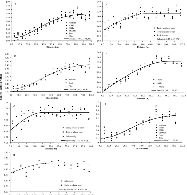
Scaled semivariograms

At each depth, semivariograms were scaled for attributes that fitted to the same model (Vieira et al.,

Altitude 10kPa 80kPa 1500kPa EAWC AWC r_b r_s Sand Silt Clay

Altitude 1

10kPa. 0.487 1

80kPa. 0.533 0.928 1

1500kPa 0.541 0.911 0.954 1

EAWC 0.053 0.491 0.130 0.192 1

AWC 0.202 0.732 0.499 0.387 0.781 1

r_b 0.077 -0.301 -0.240 -0.240 -0.238 -0.278 1

r_s -0.003 -0.114 -0.068 -0.038 -0.144 -0.194 0.249 1

Sand -0.514 -0.845 -0.863 -0.827 -0.231 -0.525 0.098 0.041 1

Silt 0.004 0.504 0.451 0.444 0.286 0.397 -0.231 -0.026 -0.661 1

Clay 0.669 0.795 0.847 0.807 0.136 0.447 -0.002 -0.062 -0.888 0.257 1

Altitude 1

10kPa. 0.501 1

80kPa. 0.503 0.891 1

1500kPa 0.499 0.920 0.937 1

EAWC 0.104 0.437 -0.019 0.169 1

AWC 0.300 0.732 0.448 0.407 0.726 1

r_b 0.103 -0.234 -0.121 -0.149 -0.277 -0.286 1

r_s 0.244 -0.023 0.033 0.046 -0.116 -0.134 0.207 1

Sand -0.502 -0.802 -0.866 -0.855 -0.050 -0.384 0.048 -0.043 1

Silt 0.155 0.336 0.355 0.358 0.036 0.162 0.081 -0.122 -0.550 1

Clay 0.530 0.655 0.792 0.726 -0.126 0.266 -0.019 0.124 -0.779 0.438 1

Altitude 1

10kPa. 0.469 1

80kPa. 0.482 0.914 1

1500kPa 0.488 0.935 0.971 1

EAWC 0.042 0.373 -0.034 0.083 1

AWC 0.273 0.787 0.519 0.519 0.759 1

r_b 0.050 -0.122 -0.018 -0.019 -0.256 -0.255 1

r_s 0.172 0.060 0.033 0.019 0.071 0.107 -0.030 1

Sand -0.521 -0.810 -0.878 -0.908 0.026 -0.367 -0.099 -0.086 1

Silt 0.246 0.550 0.553 0.609 0.075 0.259 0.191 0.117 -0.792 1

Clay 0.570 0.821 0.907 0.918 -0.061 0.378 0.042 0.053 -0.937 0.536 1

Table 3 - Correlation matrix of soil attributes, lower triangles.

(10)

1997). Figure 5 shows the scaled semivariograms for these variables, at depths 0.0–0.1 (5a and 5b), 0.1– 0.2 (5c, 5d and 5e), and 0.2–0.3 m (5f and 5g), re-spectively. At the depth of 0.0–0.1 m (Figure 5a), clay and sand fraction contents, water retention at 10, 80 and 1,500 kPa, and altitude were clustered into the same graph, since they fitted to the Gaussian model. Semivariograms similarity showed that those variables had similar patterns for spatial variability, reaching the range of 80m. The greatest difference could be ob-served in the parabolic portion close to the origin (20 meters), as a consequence of the major nugget effect of the soil physical attributes. At the depth of 0.2–0.3 m (Figure 5f), the same attributes were grouped in a similar way, but both the nugget effect and the range of the fitted model were greater than values observed for the 0.0–0.1 m. It is suggested that, despite spatial dependence increases at depth of 0.2–0.3 m (range of 86,1 meters), there was an increase in the erratic com-ponent of the semivariance, especially for water re-tention at 10, 80 and 1,500 kPa, which showed greater

source of errors due to the use of undisturbed soil samples for the laboratorial procedure on water extrac-tion with Richards membrane.

Figures 5b, 5e and 5g show results for EAWC, AWC and soil bulk density, at depths 0.0–0.1, 0.1–0.2 and 0.2–0.3 m, respectively. Differently of former variables with Gaussian model, there is not a clear similarity in the variability pattern of those at-tributes. At the three depths the spherical model was fitted, with a range between 40 and 60 m. Spatial de-pendence was found to be smaller at depths 0.1–0.2 and 0.2–0.3 m. There was a smaller grouping of at-tributes with semi variance data for the fitted mod-els, especially for the nugget effect of soil bulk den-sity at depth 0.0–0.1 m (Figure 5b), and EAW at depth 0.1–0.2 m (Figure 5e).

Altitude, sand and clay fractions semivariograms at 0.1–0.2 m the depth were grouped into the same graph (Figure 5c). Similarly to 0.0–0.1 m the depth, those attributes fitted the Gaussian model, with a range of approximately 90 m, and greater

er-Figure 6 - Experimental and fitted theoretical cross-semivariograms for altitude and soil physics attributes at 0.0–0.1 m depth. -10.00

-9.00 -8.00 -7.00 -6.00 -5.00 -4.00 -3.00 -2.00 -1.00 0.00

0.0 10.0 20.0 30.0 40.0 50.0 60.0 70.0 80.0 90.0 100.0

Distance (m)

Sand x Altitude

Gaus (0, -8.6, 87)

0.00 1.00 2.00 3.00 4.00 5.00 6.00 7.00 8.00 9.00

0.0 10.0 20.0 30.0 40.0 50.0 60.0 70.0 80.0 90.0 100.0

Distance (m)

Clay x Altitude

Gaus (0, 8, 87)

0.00 1.00 2.00 3.00 4.00 5.00 6.00

0.0 10.0 20.0 30.0 40.0 50.0 60.0 70.0 80.0 90.0 100.0

Distance (m)

10 kPa x altitude

Gaus (0, 4.85,87)

0.00 1.00 2.00 3.00 4.00 5.00 6.00

0.0 10.0 20.0 30.0 40.0 50.0 60.0 70.0 80.0 90.0 100.0

Distance (m)

80 kPa x Altitude

Gaus (0, 5.1, 87 )

0.00 0.50 1.00 1.50 2.00 2.50 3.00 3.50 4.00 4.50

0.0 10.0 20.0 30.0 40.0 50.0 60.0 70.0 80.0 90.0 100.0

Distance (m)

1500 kPa x Alitude

(11)

rors of the semi variances in relation to the model fit-ted in the parabolic portion (upper 20 m), as a conse-quence of the major nugget effect found for the sand and clay. Water retention at field capacity, 80 kPa and PWP (Figure 5d), differently of observed at depths 0.0– 0.1 m and 0.2–0.3 m, were grouped in to one graph with a spherical model. The similarity in how those attributes vary must be emphasized. It is evidenced by the greater grouping of semi variance data according to the fitted model, and by small differences in nug-get effect and range.

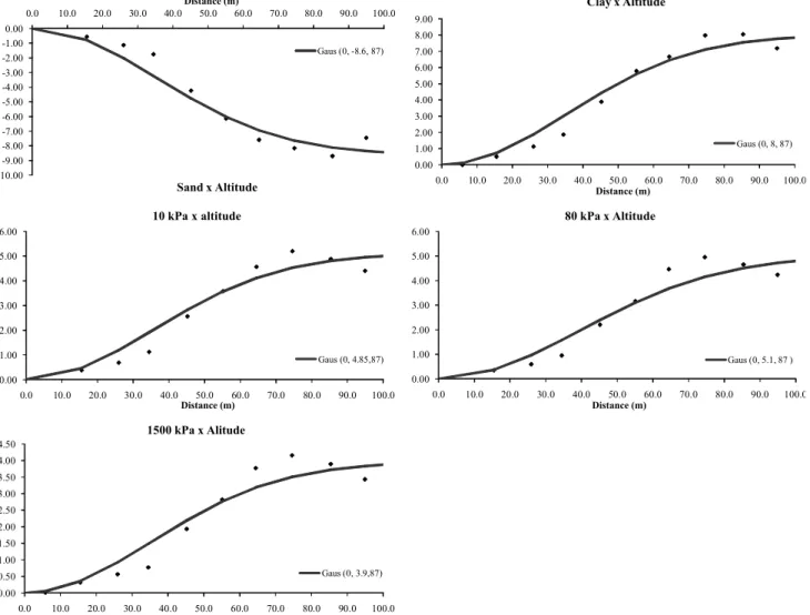
Correlation between soil attributes and cross-semivariograms

Table 3 shows Pearson correlation coefficients between all the variables. Correlation between altitude and sand and clay fraction contents was found to be significant, as well as, between altitude and water re-tention at 10, 80 and 1,500 kPa. Coefficients showed a tendency to decrease as depth increased, suggest-ing that effects of height on soil physical attributes may

decrease as soil depth increases. The results agree with the pattern observed in scaled semivariograms, i.e., al-titude and some physical-hydric attributes show a simi-lar variability pattern, presenting a trend for a decrease as soil depth increases.

In the coastal low hills of Rio de Janeiro State, soils are predominantly formed by material originated of in situ weathering of Precambrian rocks (leuco and mesocratic gneisses), and of their derived colluvial and alluvial sediments (Silva et al., 2001). On the top and the upper third of the slopes the ma-terials are usually loamy or clayey textured; on the lower section of the slope, and some of the lowlands, sandy colluvial sediments are dominant on the sur-face, and stratified sediments are a characteristic of the alluvial sites. The sediments with high sand con-tents in the lowlands may explain the negative corre-lation between altitude and sand fraction content, as well as the negative correlation of sand content with water retention at 10, 80 and 1,500 kPa, and with water availability.

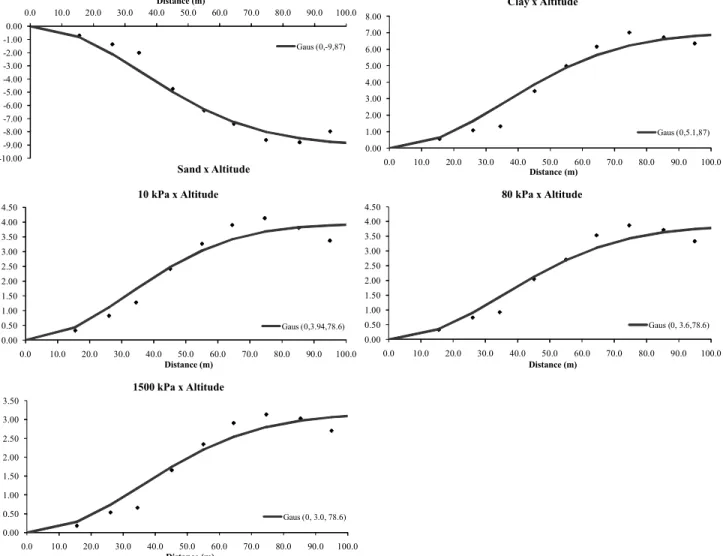
Figure 7 - Experimental and fitted theoretical cross-semivariograms for altitude and soil physical attributes at 0.1–0.2 m depth. -10.00

-9.00 -8.00 -7.00 -6.00 -5.00 -4.00 -3.00 -2.00 -1.00 0.00

0.0 10.0 20.0 30.0 40.0 50.0 60.0 70.0 80.0 90.0 100.0

Distance (m)

Sand x Altitude

Gaus (0,-9,87)

0.00 1.00 2.00 3.00 4.00 5.00 6.00 7.00 8.00

0.0 10.0 20.0 30.0 40.0 50.0 60.0 70.0 80.0 90.0 100.0

Distance (m) Clay x Altitude

Gaus (0,5.1,87)

0.00 0.50 1.00 1.50 2.00 2.50 3.00 3.50 4.00 4.50

0.0 10.0 20.0 30.0 40.0 50.0 60.0 70.0 80.0 90.0 100.0

Distance (m) 10 kPa x Altitude

Gaus (0,3.94,78.6)

0.00 0.50 1.00 1.50 2.00 2.50 3.00 3.50 4.00 4.50

0.0 10.0 20.0 30.0 40.0 50.0 60.0 70.0 80.0 90.0 100.0

Gaus (0, 3.6,78.6)

0.00 0.50 1.00 1.50 2.00 2.50 3.00 3.50

0.0 10.0 20.0 30.0 40.0 50.0 60.0 70.0 80.0 90.0 100.0

(12)

Coefficients of correlation were found to be greatest between water retention at 10, 80 and 1,500 kPa, which were also found to be strongly correlated with sand and clay fraction contents. At depths 0–0.1 m and 0.1–0.2 m, the water content at field capacity (80 kPa) and permanent wilting point were more strongly correlated with sand content. As for the depth 0.2–0.3 m, there was a greater correlation with the clay content. This pattern may result from the fact that clay content in the soil increases with depth. Despite this increase being considered small, it was responsible for the greatest errors (minimum and maximum values -Table 1).

In addition of being the most used statistical tool to evaluate the relationship between two vari-ables, the coefficient of correlation is also used in geostatistic to improve data interpolation. Because of the highly significant coefficients of correlation, cross semivariograms were performed to compare the most interesting and harder to determine (principal vari-ables) physical-hydric attributes with altitude

(auxil-iary variable). Cross-semivariograms are applied to analyze data because auxiliary variables, especially those correlated with a principal variable, may improve their estimation (Isaaks & Srivastava, 1989). Figures 6, 7 and 8 present cross-semivariograms between al-titude and sand and clay fraction contents, and be-tween altitude and water retention at 10, 80 and 1,500 kPa, at depths 0.0–0.1, 0.1–0.2 and 0.2–0.3 m, re-spectively. At depths 0.0–0.1 and 0.1–0.2 m (Figures 6 and 7) altitude may be used as a secondary vari-able, both for sand and clay, and also for water re-tention at 10, 80 and 1,500 kPa. At depth 0.2–0.3 m, this tool was found to be viable only for sand and clay contents (Figure 8). All the cross-semivariograms fitted to both Gaussian model and pure nugget effect. The smaller nugget effect, when compared to indi-vidual semivariograms of physical-hydric attributes, showed a greater spatial continuity in short distances, which is expected for variables with strong linear cor-relation (Paz-González et al., 2000). At the depth of 0.0–0.1 m, all the cross-semivariograms showed the

Figure 8 - Experimental and fitted theoretical cross-semivariograms for altitude and soil physical attributes at 0.2–0.3m depth. -16.00

-14.00 -12.00 -10.00 -8.00 -6.00 -4.00 -2.00 0.00

0.0 10.0 20.0 30.0 40.0 50.0 60.0 70.0 80.0 90.0 100.0

Distance, meters

Sand x Altitude

Gaus (0, 11.9, 80)

-12.00 -10.00 -8.00 -6.00 -4.00 -2.00 0.00

0.0 10.0 20.0 30.0 40.0 50.0 60.0 70.0 80.0 90.0 100.0

Distance (m)

Sand x Altitude

Gaus (0, 11.9, 80)

0.00 1.00 2.00 3.00 4.00 5.00 6.00 7.00 8.00 9.00

0.0 10.0 20.0 30.0 40.0 50.0 60.0 70.0 80.0 90.0 100.0

Distance (m) Clay x Altitude

Gaus (0, 7.9, 90)

-0.20 -0.10 0.00 0.10 0.20 0.30 0.40 0.50 0.60 0.70 0.80

0.0 10.0 20.0 30.0 40.0 50.0 60.0 70.0 80.0 90.0 100.0

-0.50 -0.40 -0.30 -0.20 -0.10 0.00 0.10 0.20 0.30 0.40 0.50

0.0 10.0 20.0 30.0 40.0 50.0 60.0 70.0 80.0 90.0 100.0

-0.20 -0.10 0.00 0.10 0.20 0.30 0.40 0.50

0.0 10.0 20.0 30.0 40.0 50.0 60.0 70.0 80.0 90.0 100.0

(13)

same range (87 m), as it was observed for sand and clay fraction contents at the depth of 0.1–0.2 m. Wa-ter retention at 10, 80 and 1,500 kPa, at the depth of 0.1–0.2 m, had a lower spatial dependence (range of 78.6 m). The lack of a cross-semivariogram between altitude and water retention at 10, 80 and 1,500 kPa, at depth 0.2–0.3 m, and the decrease of range with depth increasing, both results agree with the respec-tive coefficients of correlation with soil depth, as well as with the characteristics of scaled semivariograms.

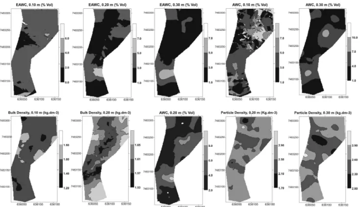
The kriged maps of all the variables, at all soil depth, are presented at figures 9 (altitude, clay con-tent and water recon-tention at 10, 80 and 1,500 kPa) and figure 10 (EAWC, AWC Bulk and Particle Density). In figure 9 it is possible to visualize the similarity be-tween spatial variability pattern of altitude and the soil physics attributes. The higher the elevation, higher the clay content as well as water retention at 10, 80

and 1,500 kPa. Besides, as soil depth increased, higher the similarity between spatial variability pat-terns of clay content and water retention at 10, 80 and 1,500 kPa, showing the high influence of tex-ture over water retention. The pattern of similarity between spatial variability observed in figure 9 is not the same in figure 10. Bulk density and particle den-sity do not follow the similar pattern of elevation and clay content, as well as, EAWC and AWC, especially at 0.0–0.1 m depth. These results are in accordance with the analysis of scaled and cross semivariograms.

CONCLUSIONS

Areas with higher elevation presented higher values of clay content, as well as, soil water retention at 10, 80 and 1,500 kPa. The correlation between al-titude and soil physical attributes decreased as soil depth

(14)

increased. The cross semivariograms demonstrated the viability in using altitude as an auxiliary variable to im-prove the interpolation of sand and clay contents to estimate data at the depth of 0.0–0.3 m, and of water retention at 10, 80 and 1,500 kPa at the depth of 0.0– 0.2 m.

REFERENCES

ADDINSOFT. XLSTAT-PLS 1.8: statistical software to MS Excel. New York: Addinsoft, 2004.

AYRES, M.; AYRES JÚNIOR, M.; AYRES, D.L.; SANTOS, A.S.

BioEstat 2.0: aplicações estatísticas nas áreas das ciências biológicas e médicas. Belém: Sociedade Civil Mamiraua/CNPq, 2003.

CAMBARDELLA, C.A.; MOORMAN, T.B.; NOVAK, J.M.; PARKIN, T.B.; KARLEN, D.L.; TURCO, R.F.; KONOPKA, A.E. Field-scale variability of soil properties in central Iowa soils. Soil Science Society of America Journal, v.58, p.1501-1511, 1994.

EMBRAPA. Centro Nacional de Pesquisas de Solos. Sistema brasileiro de classificação de solos. 2 ed. Rio de Janeiro: Embrapa Solos, 2006 605p.

EMPRESA BRASILEIRA DE PESQUISA AGROPECUÁRIA -EMBRAPA. Manual de métodos de análise de solo. Rio de Janeiro: Embrapa, 1997. 247p.

EMPRESA BRASILEIRA DE PESQUISA AGROPECUÁRIA – EMBRAPA. Levantamento semidetalhado dos solos da área do Sistema Integrado de Produção Agroecológica (SIPA) - km 47 - Seropédica, RJ. Rio de Janeiro: Embrapa Solos, 1999. 93p. (Boletim de Pesquisa, 5).

GOOVAERTS, P. Geoestatistics in soil science: state-of-the-art and perspectives. Geoderma, v.89, p.1-46, 1997.

JOURNEL, A.G. ; HUIJBREGTS, C.H.J. Mining geoestatistics. London: Academic Press, 1978. 600p.

ISAAKS, E.H.; SRIVASTAVA, R.M. Applied geoestatistics. Oxford: Oxford University Press, 1989. 560p.

KREZNOR, W.R.; OLSON, K.R.; BANWART, W.L.; JOHNSON, D.L. Soil, lanbulk densitycape, and erosion relationships in a northwest Illinois watershed. Soil Science Society of America Journal, v.53, p.1763-1771, 1989.

MALLANTS, D.; BINAYAK, P.M.; DIEDERIK, J.; FEYEN, J. Spatial variability of hydraulic properties in a multi-layered soil profile. Soil Science, v.161, p.167-181, 1996.

McBRATNE Y, A.B.; WEBSTER, R. Choosing functions for semi-variograms of soil properties and fitting them to sampling estimates. Journal Soil Science, v.37, p.617-639, 1 9 8 6 .

NOVAES FILHO, J.P.; COUTO, E.G.; OLIVEIRA, V.A.; JOHNSON, M.S.; LEHMANN, J.; RIHA, S.S. Variabilidade especial de atributos físicos de solo usada na identificação de classes pedológicas de microbacias na Amazônia meridional.

Revista Brasileira de Ciência do Solo, v.31, p.91-100, 2 0 0 7 .

PACHEPSKY, Y.A.; TIMLIN, D.J.; RAWLS, W.J. Soil water retention as related to topographic variables. Soil Science Society of America Journal, v.65, p.1787- 1795, 2001.

PAZ–GONZÁLEZ, A.; VIEIRA, S.R.; TABOADA CASTRO, M. The effect of cultivation on the variability of selected properties of an umbric horizon. Geoderma, v.97, p.273-292, 2000. REZAEI, S. A.; GILKES, R. J. The effects of lanbulk densitycape

attributes and plant community on soil physical properties in rangelanbulk density. Geoderma, v.125, p.145-154, 2005. SILVA, M.B.; ANJOS, L.H.C.; PEREIRA, M.G.; NASCIMENTO,

R.A.M. Estudo de toposseqüência da baixada litorânea fluminense: efeitos do material de origem e posição topográfica.

Revista Brasileira de Ciência do Solo, v.25, p.965-976, 2001.

(15)

SOIL SURVEY STAFF. Soil taxonomy: a basic system of soil classification for making and interpreting soil surveys. 2 ed. Washington D.C.: USDA/NRCS, 1999, p.869 (Agricultural Handbook, 436)

SOUZA, C.K.; MARQUES JÚNIOR, J.; MARTINS FILHO, M.V.; PEREIRA, G.T. Influência do relevo na variação anisotrópica dos atributos químicos e granulométricos de um Latossolo em Jaboticabal - SP. Engenharia Agrícola, v.23, p.486-495, 2003. SOUZA, Z.M.; MARQUES JÚNIOR, J.; PEREIRA G.T. Variabilidade espacial de atributos físicos do solo em diferentes formas do relevo sob cultivo de cana-de-açúcar. Revista Brasileira de Ciência do Solo, v.28, p.937-944, 2004.

TRANGMAR, B.B.; YOST, R.S.; UEHARA, G. Application of geostatistics to spatial studies of soil properties. Advances in Agronomy, v.38, p.45-93, 1985.

VAUCLIN, M.; VIEIRA, S.R.; VAUCHAUD, G.; NIELSEN, D.R. The use of cokringing with limited field soil observation. Soil Science Society of America Journal, v.47, p.175-184, 1983. VIEIRA, S.R.; HATFIELD, J.L.; NIELSEN, D.R.; BIGGAR, J.W. Geostatistical theory and application to variability of some agronomical properties. Hilgardia, v.51, p.1-75, 1983.

Received May 25, 2007 Accepted August 29, 2008

VIEIRA, S.R.; TILLOSTSON, P.M.; BIGGAR, J.W.; NIELSEN, D.R. The scalling of semivariograms and the kriging estimation.

Revista Brasileira de Ciência do Solo, v.21, p.525-533, 1997.

VIEIRA, S.R. Geoestatística em estudos de variabilidade espacial de solos. In: Sociedade Brasileira de Ciência do Solo. Tópicos avançados em Ciência do Solo. Viçosa: SBCS, 2000. 53p. WALKLEY, A.; BLACK, I.A. An examination of the Degtjareff

method of determining soil organic matter and a proposed modification of the chromic acid titration method. Soil Science, v.37, p.29, 1934.

WEBSTER, R. Is soil variation random? Geoderma, v.97, p.149-163, 2000.