A cost prediction model for machine operation in multi-field production systems

ABSTRACT: Capacity planning in agricultural field operations needs to give consideration to the operational system design which involves the selection and dimensioning of production com-ponents, such as machinery and equipment. Capacity planning models currently onstream are generally based on average norm data and not on specific farm data which may vary from year to year. In this paper a model is presented for predicting the cost of in-field and transport opera-tions for multiple-field and multiple-crop production systems. A case study from a real production system is presented in order to demonstrate the model’s functionalities and its sensitivity to pa-rameters known to be somewhat imprecise. It was shown that the proposed model can provide operation cost predictions for complex cropping systems where labor and machinery are shared between the various operations which can be individually formulated for each individual crop. By so doing, the model can be used as a decision support system at the strategic level of manage-ment of agricultural production systems and specifically for the mid-term design process of sys-tems in terms of labor/machinery and crop selection conforming to the criterion of profitability. Keywords: machinery management, decision support system, strategic management, binary programming

1_{University of Turin − Dept. of Agricultural, Forest and Food} Sciences, Largo Paolo Braccini, 2 − 10095 − Grugliasco, TO − Italy.

2_{University of São Paulo/ESALQ − Biosystem Engineering} Dept., Av. Pádua Dias, 11 − 13418-900 − Piracicaba, SP − Brazil.

*Corresponding author <remigio.berruto@unito.it>

Edited by: Dionysis Bochtis

A cost prediction model for machine operation in multi-field production systems

Alessandro Sopegno1_{, Patrizia Busato}1_{, Remigio Berruto}1_{*, Thiago Libório Romanelli}2

Received July 29, 2015 Accepted November 13, 2015

Introduction

Agricultural production adheres to intensification and extensification trends leading, on the one hand, to diversity of resource allocation and cropping practices and, on the other, to an increased geographic dispersion of fields dedicated to crop production. The diversity of management practices requires a tailored decision mak-ing process at both the strategic and the tactical man-agement levels. Existing information and decision sup-port systems provide a number of services to farmers. However, these services use closed specifications and do not provide the farmers with the ability to tailor their systems according to their practical needs (Sørensen et al., 2010; Kaloxylos et al., 2014). In addition to the diver-sification of management, increasing geographic disper-sion also leads to the engagement of farmers in supply chain activities, especially in the case of biomass pro-duction. However, such an engagement provides cost-effective solutions for supply chain activities which can increase farm business income and, additionally, reduce the ownership cost of machinery due to increased usage (Tatsiopoulos and Tolis, 2003).

Therefore, new tools for different planning levels should be made available to farmers that also include logistics management functionalities (Sørensen and Bochtis, 2010), especially when considering logistics op-erations as an inseparable part of the production system, capacity planning is a central task in the farm manage-ment process as well as a prerequisite for operations scheduling (Orfanou et al., 2013; Bochtis et al., 2013). Capacity planning considers the system design involv-ing the selection of production components, such as the selection and dimensioning of machinery and equip-ment, taking into account the operational demands, resource availability, potential working methods, and

the associated cost (Bochtis et al., 2014). A number of studies focusing on machinery capacity planning have been conducted (e.g. Berruto and Maier, 2001; Søgaard and Sørensen, 2004; Sahu and Raheman, 2008; Busato et al., 2013; Busato and Berruto, 2014; Busato, 2015). How-ever, planning in general is based on average norm data and not on specific farm data that may vary from year to year. To address this concern, a model is presented in this paper on the cost prediction of in-field and transport operations for multiple-field and multiple-crop produc-tion systems. The proposed model refers to the strategic level of decision making in an agricultural production system pertaining to the design of the labor/machinery system in connection with the types of crops selected.

Materials and Methods

Model overview

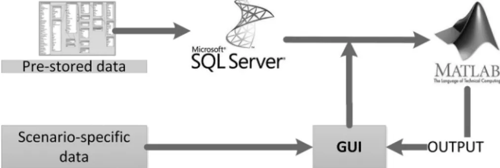
being inserted by the user and also to provide a sugges-tion for the parameters that might not be available for a particular scenario. The scenario-specific data as regards input data such as machinery dimensioning (e.g. operat-ing width and power), crop allocation, field features (e.g. area), network distances (e.g. distances between fields and distances of each field to the delivery facility), op-erational data (e.g. working speeds), and monetary costs (e.g. fuel cost and labor wages). All the processing of data takes place in the MATLAB environment. This au-tomated procedure allows for a comparison of operation-al time and totoperation-al costs of many scenarios that differ in terms of parameter (e.g. working speed) without having to insert all data from scratch.

Model inputs

Fields and crop related data

Let F = {1, 2, 3…} and C = {1, 2, 3…} represent the set of fields which constitutes the cultivation area of the system (e.g. a farm) and the set of crops that is cultivated in the production system, respectively. The numerical input parameters for each individual field include the area of each field, a_i, i

∈

F, the width of the field area (assuming a rectangular field shape), xi,

i ∈ F, the distance from the delivery facility (depot or bioenergy production plant), di, i ∈ F, and the average

speed for a transport operation between the field and the farm,si

tr

, i ∈ F. Finally, the classifying of soil workabil-ity, Wor_i = {1, 2, 3…}, i

∈

F, is based on three classes that correspond to a dimensionless soil texture adjustment parameter: 1, fine; 2, medium, and 3, coarse texture soils (ASAE, 2009a). Soil workability is needed for the selec-tion of coefficients from the database for estimating the variables related to in-field machinery performance.

A crop can be allocated to different fields and con-versely, in a field a number of crops can be allocated. This fact results in a clustering of the production system area that is described by a F |×|C| matrix A in which element a_ijprovides the area of the field i ∈ F allocated to crops j ∈ C (a_ij = 0 if crop j is not cultivated in field

i

_{; individual field area:}ai a

f ij j C

= ∈

∑

; total area allocated to a crop c

j ij i F

a a

∈

=∑ _{; total production area}

,

ij i F j C

a a

∈ ∈

= _{∑ ).} Further-more, a binary decision function cf i j C F( , ) : × 

{ }

0,1 is

defined where cf(i, j) = 1 if crop i is cultivated in field j, and cf(i, j) = 0 otherwise. Each production area of a field in which an individual crop is cultivated will be referred to as a “production unit” (the number of pro-duction units in the propro-duction system is equal to the number of non-zero elements of the previously de-fined matrix, or equivalent to the cardinality of the set: |{aij / i ∈ F, j ∈ C, aij, ≠ 0}|.

Resources related input

In a production system different types of labor could be involved, for example: family people, seasonal, specialized, etc., with a different hourly cost and produc-tivity level. Let L = {1, 2, 3, …} represent the set of the different types of labor. A cost, ci

l

, i ∈ L is assigned to each labor type.

Let T = {1, 2, 3, …} represent the set of available tractors. Each tractor i ∈ T is characterized by the values of cost, t

i

c , power, t i

p , and time used for other activi-ties not related to the production system under consid-eration, t

i

u . The vehicle type (2-wheel drive or 4-wheel drive) is defined by the following binary parameters

{ }

2

0,1

WD i

vt ∈ and 4

{ }

0,1

WD i

vt ∈ (note that the following condition stands: 4

{ }

{

2

}

0,1 \

WD WD

i i

vt ∈ vt ).

Let M = MNMF∪ MIMF∪ MOMF represent the machinery

set where M_NNF = {1, 2, 3,…}, MIMF =

{

MNMF,MNMF +1,...

}

, and MOMF=

{

MIMF,MIMF +1,...

}

represents the sub-sets of the machinery dedicated to neutral material flow operations (there is neither material addition nor ma-terial removal to/from the field, e.g. tillage, mowing, etc.), to input material flow operations (where a quan-tity of a ‘‘commodity’’ is transported by the machine and is distributed in the field area, e.g., seed, fertil-izer, etc.), and output material flow operations (where a quantity of a ‘‘commodity’’ is transported out of the field area, e.g., harvesting), respectively (according to the terminology found in Bochtis and Sørensen, 2009). The set of the self-propelled machines is represented byMSP⊆M. A machine is identified by the values of

purchasing cost m,

i

c i∈M, working width m,

i w i∈M, hourly use for other activities m,

i

u i∈M, hopper capac-ity cap ii, ∈MIMF∪MOMF, in the case of input and output

material flow operations, and power m,

i SP

p i∈M in the case of self-propelled machines. Furthermore, a labor

type is allocated to each machine. This allocation gener-ates the binary decision function lm i j( , ) :L M× 

{ }

0,1 where lm(i, j) = 1 if labor type i is assigned to machinery j, and lm(i, j) = 0 otherwise.

Let P = {1, 2, 3…} represent the set of the pro-ductive means. Each propro-ductive mean is identified by the value of the cost p,

i

c i∈P. For the allocation of a productive mean to each production unit the binary function pfc i j k P( , , ) : × ×F C_

{ }

0,1 is defined. Each el-ement of the function domain is associated with the value 1 (in the case where the productive mean i is applied to the k crop cultivated in the field j) or 0 (otherwise).

Operation functions

Operational data with regard to information re-lated to field and transport operations, the allocation of machinery to them, and the assignment of these operations to the different production units. In the operations data set, a set of operations is generated,

{

1,2,3,...

}

O= . Each operation o_i, i∈ O is characterized by the vector: oi→

{ } { } { }

m , j , k OF, i , that describes the

se-lected “entities” related to the specific operation, where

( )

{

}

, , , i , 1

m∈T j∈M k∈C OF ⊆ x∈F cf k x = . The input numerical parameters are the operating speed op,

i s i∈O, the working width e,

i

w i∈O, the number of repetitions (passes) rep,

i

n i∈O, the skipped area op,

i

sk i∈O (an in-teger number providing the field-work tracks that are skipped between two sequential track traversals of the machine; zero value corresponds to complete area cov-erage), the number of the workers/operators commit-ted to the operation op,

i

l i∈O, and the labor coefficient ,

op i

lco i∈O. The working width that is entered in the operations data set is not necessarily the same as the one in the machinery data set. The former provides the effective working width 1

,

i

o i e th

w ≤w i∈O. The pre-stored database, however, provides as default the number of the theoretical working width for various items of equip-ment.

In the current presentation, for reasons of sim-plicity, it has been assumed that when an operation is assigned to a specific crop and specific field, the opera-tion relates to all of the area of the field allocated to the cultivation of that crop. Consequently (since a_ijprovides the area of the field i∈ F that is allocated to crop j∈ C) in each field the operations is carried out in the area:

,i3, , i

j o

a i∈O i∈OF), the total area subjected to the opera-tion in quesopera-tion is ,i3

i j o j OF a ∈

∑

_).

The decision functions involved in the opera-tions include: to i j T O( , ) : × 

{ }

0,1 , depending on whether tractor i ∈ T is assigned to operation i ∈ O,

{ }

( , ) : 0,1

mo i j M O×  , or if machine i∈ M is assigned to operation i∈ O, and ocf i j K( , , ) :O C× ×F_

{ }

0,1 , de-pending on whether operation i∈O is assigned to crop j∈ C cultivated in field k∈ F.

Analogously, in the case of field operations, a set of transport operations,H=

{

1,2,3,...

}

, is gener-ated, and each transport operation is symbolized as h_i,

i ∈ H. A transport operation is characterized by a ve-tor hi→

{ } { } { }

m , j , c HF, i , which describes the

select-ed “entities” relatselect-ed to the transport operation, where

( )

{

}

, , , i , 1

m T j∈ ∈M k∈C HF ⊆ x∈F cf k x = . The nu-merical parameters inputted are the transport speed,

,

tr i

s i∈H, the total quantity, tr,

i

q i∈H , the loading/un-loading time in the field 1

,

i

lu i∈H, the loading/unload-ing time in the farm (or plant), 2

,

i

lu i∈H, the number of the workers/operators committed to the transport tasks,

,

tr i

l i∈H, and the labor coefficient tr,

i lco i∈H.

Analogously, as in the case of field opera-tions the following decision funcopera-tions are defined:

( )

, :

{ }

0,1

th i j T O× _ , depending on whether trac-tor i ∈ T is assigned to transportation operation i∈ H,

( )

, :

{ }

0,1

mh i j M×H ,or if machine i∈ M is assigned to operation i∈ H, hcf i j k

(

, ,

)

:O C F× × 

{ }

0,1,or if op-eration i∈ H is assigned to crop j∈ C _{cultivated in field} k∈ F.

External services and income functions

For this function different types of external services are selected. Let S={1, 2, 3,…} represent the set of poten-tial external services to the production system. For each service type i∈ S , a cost, s

i

c is assigned. For the allocation of an external service to each production unit the function

(

, ,

)

:

{ }

0,1

sfc i j k s F C× × _ was defined. Each element of the function domain is associated with the value 1, in cas-es where the service i is applied to the k crop cultivated in the field j, or 0 otherwise, during the repeated assignment of services to production units as an input to the system. The total area of the production system where an external service i is applied is given by:

,

( , , ) jk j F k C

scf i j k a

∈ ∈

⋅

∑

.

Income can be derived either from product sales or from subsidies for the specific product. For each type of crop a number of sub-products could be cultivated for profit; for example, the grain, the straw, crop resi-dues, etc. Let sP_i = {1, 2,…} represent the set of po-tential products from the cultivation of crop i∈ C. For each one of the sub-products from each crop the val-ues of the sale price and the subsidy (if any) per unit are inserted into the system, symbolized by c

ij c and

c ij

c , i ∈ C, i ∈ sP_i, respectively. For the allocation of a sale action and the corresponding subsidy for a sub-product of a sub-production unit the following functions are introduced: in cf i j k1

(

, ,

)

:C sP× i×F

{ }

0,1 and

(

)

{ }

2 , , : i 0,1

in cf i j k C sP× ×F , respectively, where in1fc(i, j, k) = 1 if the sub-product jof crop i that is cul-tivated in field k is sold; otherwise 0.

Processes

Operational time

For an operation o_i in the cropped area j∈ OF_i the operational time is the summation of the effective time and the turning time: turn

i

t , where

0 3i

op e op i i turn

is the time that is allocated to turnings and is a function of the number of turns that a machine has to execute for a given operating width and given field dimensions. The transport time for a transportation operation on hi for

the material removal from the cropped area j∈ HF_i can be written as:

1 2 2 2 i tr j tr i

i tr i i

i h

d q

t lu lu

cap s

⋅

 

= _ + + _

 

It should be noted that for the same crop in differ-ent areas allocated it is not necessary to assign the same operations (for example, different farm practices can be followed for the same crop cultivated in different fields). Nevertheless, in the current study, it is assumed that for a specific crop the set of operations are identical for all the fields where this crop has been established (analo-gously in the case of transport operations). Under this assumption OFi≡HFi ≡

{

x∈F cf k x( , ) 1=

}

.

Variable costs

The variable cost for the execution of an operation includes labor, fuel, and repair and maintenance costs. The labor cost for an operation is estimated based on the assignment of labor type to the machine which carried out the specific operation and the associated hourly cost. For an individual operation o_i∈ O can be written as:

( , ) ( , ) l op k i j M

k L

mo j i lm k j c t

∈ ∈

⋅ ⋅ ⋅

∑

Analogously, the labor cost in the case of a trans-port operation hi, i∈ H can be written as:

( , ) ( , ) l op k i j M

k L

mh j i lm k j c t

∈ ∈

⋅ ⋅ ⋅

∑

For the calculation of accumulated repair and maintenance costs, the following equation given by the Agricultural Machinery Management Data ASAE Stan-dard, (ASAE, 2009b) was used:

(

)

2 1

1 1000 t i RF t

t t t i

i i i t t

i i a

rmc RF c

a u

 

= ⋅ _{ } ⋅

−

 

where, t i

rmc is the hourly repair and maintenance cost for typical field operating speeds of the tractor i ∈ T, (€_{), 1}t

i

RF and 2t i

RF are repair and maintenance factors (ASAE, 2009a), and t

i

a is the accumulated use of trac-tor (h). Analogously the maintenance cost m

i

rmc of a ma-chine i∈ M is estimated.

The repair and maintenance cost for a field opera-tion o_i∈ O can be written as:

( , ) t ( , ) m op

j k i

j T k M

to j i rmc mo k i rmc t

∈ ∈

 ⋅ + ⋅ ⋅

 

∑

and for a transport operation h_i, i∈ H as: ( , ) t ( , ) m tr

j k i

j T k M

th j i rmc mh k i rmc t

∈ ∈

 ⋅ + ⋅ ⋅

 

∑

The fuel cost

(

op, , tr,

)

i i

fc i∈O fc i∈H for an

opera-tion o_i∈ O is given by: op op i i

fc ⋅t , while the fuel cost for a transport operation hi, i∈ H is given by:

tr tr i i fc ⋅t . For fuel consumption estimation, the equation regarding the measure of specific volumetric fuel consumption given at Agricultural Machinery Management Data ASAE Standard (ASAE, 2009a) was used:

(

264 391 0203 738 173

)

pto Q= X+ − X+ ⋅X P⋅

where, Q is the diesel fuel consumption at partial load for operation (l/h), X = P/P_rated is the ratio of equivalent power-take-off (PTO) power, P, required by the opera-tion to the rated PTO power, P_rated, that is considered as 83 % of the gross fly wheel. The equivalent PTO power is calculated by: P = P_db /(E_mE_t)+ P_pto , where E_m is the mechanical efficiency of the transmission and power train, typically 0.86 for tractors with gear transmission (this number is used by the system), E_t provided by the system’s data base (built upon ASAE (2009a) clause 3, table provided), P_pto is the PTO power required by the implement (kW), and P_dbthe drawbar power required for the implement. The former power requirement is given by P_pto = a + b.w + cf, where a, b, c are machine spe-cific parameters (ASAE (2009a) Table 2), w the working width, and F → t/h the material feed, while the latter is calculated using: P_db = D.s/3.6, where the implement draft, D, is computed using a different approach for field and transport operation cases.

Table 1 − Characteristics of the different fields considered in the system.

Field ID 1 2 3 4 5 6 7

Crop Wheat Wheat Wheat Wheat Corn Corn Corn

Area (ha) 13 13 9 6 15 10.5 25

Width (m) 260 130 180 100 250 70 500

Distance (km) 1 1 5 5 10 10 13

Transport speed

(km h−1₎ 20 20 25 25 30 30 30

Workability medium medium coarse coarse fine fine fine

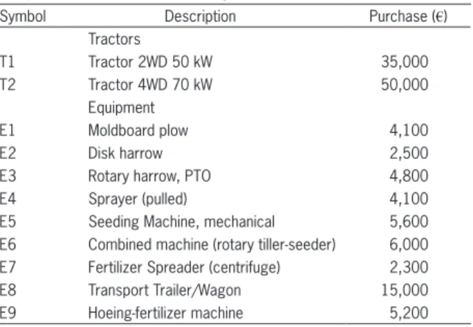
Table 2 − Characteristics and purchase price of tractors and equipment considered in the system.

Symbol Description Purchase (€₎

Tractors

T1 Tractor 2WD 50 kW 35,000

T2 Tractor 4WD 70 kW 50,000

Equipment

E1 Moldboard plow 4,100

E2 Disk harrow 2,500

E3 Rotary harrow, PTO 4,800

E4 Sprayer (pulled) 4,100

E5 Seeding Machine, mechanical 5,600

E6 Combined machine (rotary tiller-seeder) 6,000 E7 Fertilizer Spreader (centrifuge) 2,300

E8 Transport Trailer/Wagon 15,000

Field operations

For the estimation of the implement draft in the case of field operations the following equation (provided in ASABE D497, 2009) was adopted:

2

i

D=Wor A_ +Bs Cs+ _⋅ ⋅w de, where parameters A, B, C(machine-specific parameters) are selected from a data base that has been constructed based on Table 1 in ASABE D497 (2009), and de is the tillage depth and is provided by the system data base that gives the sug-gested tillage depth for each type of operation.

Transport operations

For the estimation of the draft requirements in the case of transport operations the following equa-tion provided in ASABE EP496 (2009) was applied: D = R_sc + MR, where R_sc is the soil and crop resistance and

MR

_{the total motion resistance. In the transport} operations, depending on the direction of travel, both the weight of the full loaded trailer and the weight of the empty trailer are considered. For the out of field transport the hard soil coefficient is considered. The total of implement motion resistance is estimated by:

M

MR=

∑

R , as the summation of each individual wheel supporting the implement which can be as-sumed as RM = 0.55m where m is the dynamic wheel

load and the 0.55 coefficient has been estimated as-suming the surface to be concrete (ASABE 497 (2009), Clause 3.2.1.1).

Model outputs

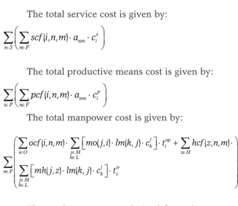
Taking into account all the previously defined functions and processes, the various cost elements can be calculated by the following equation. The total opera-tions cost is given by:

( , , ) ( , ) ( , )

( , , ) ( , ) ( , )

t m op op

j k i i

i O j T k M

t m h h

n F _{j k z z}

Z H j T k M

ocf i n m to j i rmc mo k i rmc fc t

hcf z n m th j z rmc mh k z rmc fc t

∈ ∈

∈

∈

∈ ∈

∈

Σ ⋅ Σ _ ⋅ + ⋅ + _⋅ +

 

 

 Σ ⋅ Σ _ ⋅ + ⋅ + _⋅ 

 

 

∑

The total service cost is given by: ( , , ) s

nm i i S n F

scf i n m a c

∈ ∈

 _{⋅ ⋅} 

 

 

∑ ∑

The total productive means cost is given by: ( , , ) p

nm i i P n F

pcf i n m a c

∈ ∈

 _{⋅ ⋅} 

 

 

∑ ∑

The total manpower cost is given by:

( , , ) ( , ) ( , ) ( , , )

( , ) ( , )

l op k i

i O j M z H

k L

l tr

n F _{k z}

j M k L

ocf i n m mo j i lm k j c t hcf z n m

mh j z lm k j c t

∈ ∈ ∈

∈

∈ ∈ ∈

 ⋅ _ ⋅ ⋅ _⋅ + ⋅

 

 

 _{ ⋅ ⋅ ⋅} 

 

 

 

 

∑

∑

∑

∑

_∑

The total expenses are derived from the summa-tion of the above elements. The margin is estimated by subtracting the total expenses cost from the total product sales and subsidies which are given by:

1 2

1 ( , , ) 2 ( , , )

m

in in

nm mi nm mi

i sP n F

in cf i m n a c in cf i m n a c

∈ ∈

 _{⋅ ⋅ + ⋅ ⋅} 

 

 

∑ ∑

Results

Case study description

To demonstrate the model’s capability, a case study that refers to a real production system located in the Piedmont region in North Western Italy, is present-ed. The production system consists of seven (7) fields of which the operational features are presented in Figure 2. The total area of the production system is 91.50 ha (1 ha = 10,000 m2_{) in which 41 ha are allocated to wheat}

pro-duction and 50.5 ha to maize propro-duction. Figure 2 pres-ents a topological configuration of the production sys-tem. Note that the field shapes represent a micrograph of the real shapes of the fields. In the specific production

system, the storage facility where biomass is transported after harvesting and handling operations is at the farm (on-farm storage of the crop/biomass). The distances of the different fields from the farm have a high variation, a fact that provides a good perception of the influence of the cost for the transportation of resources and the movement of equipment from farm to field, and for the transportation of the crop/biomass form field to farm.

Once the fields and equipment are inserted, the user, in order to complete the field operations, should add the productive means costs. The productive means used by the farmer include: Potassium Chloride 2006; Ammo-nia Nitrate; Enesco; Logran; Aqua/Water; Urea; Potassium Chloride; Corn-seed hybrid; Mikado; and Ghibli. The cur-rent commercial price and the dosage of each individual input are provided from the pre-stored data base.

Once the tractors, equipment, and productive means are inserted, the user was able to proceed to en-ter the field operations and the logistic operation. Figure 3 presents the allocation of the various equipment and tractors to the selected field operations for both maize and wheat crops, as well as the operating width of equip-ment and the working speed of the tractors. For all of the transport operations (maize crop, wheat grain, and wheat straw) the tractor with the higher power (Tractor 4WD 70 kW) combined with transport trailer equipment was committed to the operation.

Table 2 lists the available tractors and equipment and their purchase price. Note that the user selects each individual machinery item from the graphical user inter-face and all the related parameters (lifetime, suggested accumulated use, repair and maintenance coefficients, etc.) are provided by the pre-stored data base.

Model implementation

The model allows for breaking down the opera-tion in a way that captures the complexity inherent in a real farm situation. Its functionality allows for each individual field to be selected for specific operations (for the same crop), different rates of input resources (e.g. fertilizer), and also, related to logistic operations, the selection of different delivery locations and distances (farm or processing plant). The output provides results per crop or per single field. All of the results per crop are the weighted average from the data from a single field.

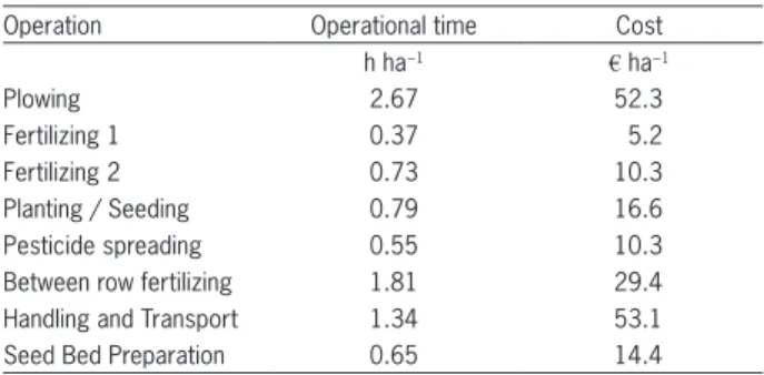
Table 3 presents in detail the average mechanical operation costs per single operation for maize produc-tion (cultivated in fields 5, 6, and 7). The three major costs are related to plowing, transport operation, and between-row fertilizing of the crop. Average expenditure for transporting the grain is as expensive as the plowing operation. This is due to the relatively long distances of the three maize fields from the delivery location (5, 10, and 13 km).

Table 4 presents the operation costs for wheat pro-duction, referring to fields 1 to 4. In the case of wheat, the logistic operations are on average less costly (34

€ _ha−1_{, including the transportation of both grain and}

straw) since the average distance from the fields is quite small compared to the fields where maize is cultivated.

Table 5 presents the summary of costs and rev-enues for both maize and wheat production. For maize the profit is 639 € _ha−1_{, the output/input ratio is 1.44 (if}

we include EU contribution). It means that for each €

spent it returned back to the producer 1.44 € _{in vendible}

product, including contribution. Operation cost accouts for approximately 13 % of the total cost. The results also provide an average production cost per t of grain which is 111 € _t−1 _{in the specific case. This considerably high}

production cost stems from the high cost of renting of land (app. 350 € _ha−1 _{according to the prevailing current}

values in the specific area) which implies 24 % of the production costs.

For wheat, the profit is approximately 532 € _ha−1

and the output/input ratio about 1.50 (if we include EU contribution). Operational cost accounts for approxi-mately 14 % of the total cost. From Figure 4 we can understand the importance of the cost of logistics and operations. Wheat crops must be collected in the form of two products, grain and straw with a resultant increase in transport costs. In fact, the logistics cost at 5 km (52

€ _ha−1_{) is comparable to the logistic cost of maize at 10}

Table 3 − Average operation costs for maize production (three fields-total of 50.5 ha).

Operation Operational time Cost

h ha−1 € _ha−1

Plowing 2.67 52.3

Fertilizing 1 0.37 5.2

Fertilizing 2 0.73 10.3

Planting / Seeding 0.79 16.6

Pesticide spreading 0.55 10.3

Between row fertilizing 1.81 29.4

Handling and Transport 1.34 53.1

Seed Bed Preparation 0.65 14.4

Table 4 − Average operation costs per wheat production cultivated on 41 ha (fields 1, 2, 3 and 4).

Operations Operational time Amount

h ha−1 € _ha−1

Seed Bed Preparation 0.60 18.3

Plowing 2.36 46.2

Fertilizing 1 (before planting) 0.41 5.8

Planting / Seeding 1.35 29.3

Fertilizing 2 (after planting 1) 0.44 6.3 Fertilizing 3 (after planting 2) 0.39 5.5

Pesticide spreading 0.36 6.7

Handling and Transport (straw) 0.33 13.8 Handling and Transport (grain) 0.67 21.2

Table 5 − Summary of average costs and revenues for wheat and maize production.

Economic parameters Wheat Maize

Operation costs (€ _ha−1_{) 153.1 191.6} Resource costs (€ _ha−1_{) 311.7 421.4} Service costs (€ ha−1_{) 598.0 829.0} Total expenses (€ _ha−1_{) 1,062.8 1,442.0} Product sales & subsidizes (€ ha−1_{) 1,595.0 2,081.0}

Profit (€ _ha−1_{) 532.2 639.0}

Output/Input ratio (€ ha−1_{) 1.50 1.44}

Unitary Costs (€ _t−1₎ straw 17.9 _110.7 grain 107.5

Figure 4 − Operations and logistics cost distribution – the numbers within the bars are in € ha−1_.

km (48 € _ha−1_{). These costs have a significant impact on}

the total operations cost since they account for between 16 % and 28 % of the total mechanical operations cost, and they are often unknown and not very well evalu-ated. The slightly less operations cost for field 7 com-pared to field 6 is due to the longer shape of field 7 since they are located at the same distance from the farm (see Figure 2). Field 7 requires less turning per ha and this implies lower operation time and costs.

The increase of distance also implies an increase in the field operations cost, because the operations in-clude transfer of equipment from field to farm as well, and this extra cost is a function of the field distance from the farm.

changes. The increased sensitivity of profit is reasonable since the yield directly and linearly affects sales income. In order to investigate further the effect of sales income and specifically of the sale price on profit, which is inherently the most important output parameter from the farmer’s perspective, the change in profit with changes in the sales price has also been investigated in the basis production scenario. Specifically, if the sales price is reduced by 10 % from the one considered in the basis scenario, profit will be reduced by 19 % for wheat production (431.1 €_{) and by 20 % for maize production}

(508.5 €_{), and if the sales price increased by 10 % from}

the one considered in the basis scenario the profit will be increased by 19 % in the case of wheat production (633.1

€_{) and by 31 % in the case of maize production (833.5} €_).

Discussion

A model for the cost prediction of in-field and trans-port operations for multiple-fields and multiple-crop pro-duction systems was presented and demonstrated in a real production system scenario. It was shown that the proposed model can deal with variability, in terms of in-put parameter values, in the production of a typical farm and provide cost predictions for complex cropping sys-tems where labor and machinery are shared between the various operations that the farm manager plans for each individual crop. By so doing, the model can be used as a decision support system at the strategic level of agricul-tural production systems and specifically for the mid-term design process of the system in terms of labor/machinery and crop selection according to the criterion of profit.

This detailed analysis of cost allows for the con-sideration of the sensitivity of the model. Any change in parameters, e.g. working speed, field distance, field shape etc., can be seen in the results, both at farm level, crop level, or at a single field level. The incidence of logistics operation, often unknown, range from 16 % for

fields nearby up to 28 % for fields more distanced from the farm. This is a very important consideration where an expansion of farm activities implies renting of new plots, and could lead to better rental agreement if the owner of the land knows the magnitude of the influence of the distance on revenues.

In Figure 4 it can be seen that for the same crop and the same field distance, a different operational cost is the result. This occurs due to the differentiation of the field shapes and areas. Although the inclusion of the field shape is rather simple in the model presented (through the consideration of only rectangular fields) there is still an effect on the results derived regarding the cost of the field operations (and consequently the to-tal cost and profit). The inclusion of complex sub-models that take into account the shape of the field independent of its geometrical complexity, the operations plan, i.e. coverage pattern (Bochtis et al., 2013), and the in-field obstacles (e.g. Zhou et al., 2014) will provide an in-depth re-presentation of the actual task times elements and consequently a more accurate estimation of the in-field operations cost contribution.

As regards the model itself, the mathematical de-scription was oriented towards the building of a number of binary decision variables, including:

( , ) : {0,1}

cf i j C F×  for the allocation of a crop to a field ( , ) : {0,1}

lm i j L M×  for the allocation of a labor type to an operation

( , , ) : {0,1}

pfc i j k P F C× ×  for the allocation of a pro-ductive mean to a crop to a field

( , , ) : {0,1}

sfc i j k S F C× × _ for the allocation of a service in a crop in a field

( , , ) : {0,1}

to i j k T O×  for the allocation of a tractor to a field operation

( , ) : {0,1}

mo i j M O× _ for the allocation of an item of equipment to a field operation

the analogous previous two in the case of transport op-erations

( , , ) : {0,1}

ocf i j k O C F× ×  for the allocation of an op-eration to a crop.

This model development approach, in combi-nation with the use of an engineering programming environment, provides the potential for the inclusion of numerous binary programming optimization mod-els (e.g. which crops are allocated to which fields, which machinery is allocated to which operations, which production means are allocated to which crop, etc.) either according to single-criterion or multiple-criteria goals. Furthermore, the pre-stored data bases

provided to the user in connection with the graphical user interface provide the potential for a web-based decision support tool. All of the above require fur-ther research in the direction of the work presented in this study.

References

American Society of Agricultural Engineers [ASAE]. 2009a. ASAE D497.6 Agricultural machinery management data. p. 360-367. In: ASAE standards. ASAE, St. Joseph, MI, USA.

American Society of Agricultural Engineers [ASAE]. 2009b. ASAE EP496.3 Agricultural machinery management. p. 354-357. In: ASAE standards. ASAE, St. Joseph, MI, USA.

Berruto, R.; Maier, D.E. 2001. Analyzing the receiving operation of different grain types in a single-pit country elevator. Transactions of the ASAE 44: 631-8.

Bochtis, D.D.; Sørensen, C.G. 2009. The vehicle routing problem in field logistics part I. Biosystems Engineering 104: 447–457. Bochtis, D.D.; Sørensen, C.G.; Busato, P. 2014. Advances in

agricultural machinery management: a review. Biosystems Engineering 126: 69-81.

Bochtis, D.D.; Dogoulis. P.; Busato, P.; Sørensen, C.G.; Berruto, R.; Gemtos, T. 2013a. A flow-shop problem formulation of biomass handling operations scheduling. Computers and Electronics in Agriculture 91: 49-56.

Bochtis, D.D.; Sørensen, C.G.; Busato, P.; Berruto, R. 2013b. Benefits from optimal route planning based on B-patterns. Biosystems Engineering 115: 389-395.

Busato, P. 2015. A simulation model for a rice-harvesting chain. Biosystems Engineering 129: 149-159.

Busato, P.; Berruto, R. 2014. A web-based tool for biomass production systems. Biosystems Engineering 120: 102-116.

Busato, P.; Sørensen, C.G.; Pavlou, D.; Bochtis D.D.; Berruto, R.; Orfanou A. 2013. DSS tool for the implementation and operation of an umbilical system applying organic fertilizer. Biosystems Engineering 114: 9-20.

Kaloxylos, A.; Groumas, A.; Sarris, V.; Katsikas, L.; Magdalinos, P.; Antoniou, E.; Politopoulou, Z.; Wolfert, S.; Brewster, C.; Eigenmann, R.; Terol, C.M. 2014. A cloud-based farm management system: architecture and implementation. Computers and Electronics in Agriculture 100: 168-179. Orfanou, A.; Busato, P.; Bochtis, D.D.; Edwards, G.; Pavlou, D.;

Sørensen, C.G.; Berruto R. 2013. Scheduling for machinery fleets in biomass multiple-field operations. Computers and Electronics in Agriculture 94: 12-19.

Sahu, R.; Raheman, H. 2008. A decision support system on matching and field performance prediction of tractor implement system. Computers and Electronics in Agriculture 60: 76-86. Søgaard, H.; Sørensen, C. 2004. A model for optimal selection of

machinery sizes within the farm machinery system. Biosystems Engineering 89: 13-28.

Sørensen, C.G.; Bochtis, D.D. 2010. Conceptual model of fleet management in agriculture. Biosystems Engineering 105: 41-50.

Sørensen, C.G.; Pesonen, P.; Fountas, S.; Suomi, P.; Bochtis, D.D.; Pedersen, S.M. 2010. A user-centric approach for information modelling in arable farming. Computers and Electronics in Agriculture 73: 44-55.

Tatsiopoulos, I.P.; Tolis, A.J. 2003. Economic aspects of the cotton-stalk biomass logistics and comparison of supply chain methods. Biomass and Bioenergy 24: 199-214.