www.scielo.br/rbg
EXPERIMENTAL DETERMINATION OF THE EFFECTIVE PRESSURE COEFFICIENTS
FOR BRAZILIAN LIMESTONES AND SANDSTONES
Guilherme Fernandes Vasquez
1, Eur´ıpedes do Amaral Vargas Junior
2,
Cleide Jeane Bacelar Ribeiro
3, Marcos Le˜ao
4and Julio Cesar Ramos Justen
5Recebido em 11 junho, 2008 / Aceito em 26 janeiro, 2009 Received on June 11, 2008 / Accepted on January 26, 2009
ABSTRACT.There are numerous efforts to obtain information about saturation and pressure changes due to reservoir production from time-lapse seismic data. In spite of some good examples existing on the literature, there are a lot of approximations behind those studies. Generally, it is assumed that the seismic properties are functions of saturation and differential pressurePd(overburden minus fluid pressure). Actually, the stress that governs the seismic behavior is the effective stressPe f,
which is not exactly equal toPd. In fact it is equal to the overburden stress minusntimes the fluid pressure. Such coefficient (n) is known as the effective stress
coefficient. Sometimes, depending on the circumstances, it might be identified as the Biot-Willis coefficient taking into consideration the bulk modulus of the porous media. In this paper, laboratory results in a tentative to quantify thenvalues for Brazilian limestones and tight sands will be presented. It is important to point out, that is the first effort to perform this sort of measurements on Brazilian rocks. The results have shown that the mentioned approximations can introduce errors on pressure estimations from time-lapse data even for high porosity rocks.
Keywords: effective pressure, porepressure, seismic velocities, Biot-Willis coefficient, 4D seismic.
RESUMO.H´a v´arios esforc¸os no sentido de obter informac¸˜oes sobre mudanc¸as de saturac¸˜ao e press˜ao, devidas `a produc¸˜ao dos reservat´orios, a partir de dados s´ısmicos com lapso de tempo. A despeito de alguns bons exemplos existentes na literatura especializada, v´arias aproximac¸˜oes s˜ao feitas para a realizac¸˜ao destes estudos. Geralmente, ´e assumido que as propriedades s´ısmicas s˜ao func¸˜oes da saturac¸˜ao e da press˜ao diferencialPd(press˜ao de soterramento menos press˜ao de
fluido). Na verdade, a tens˜ao que determina o comportamento s´ısmico ´e a tens˜ao efetivaPe f, que n˜ao ´e exatamente igual aPd. De fato, esta ´e igual `a tens˜ao de
soterramento menosnvezes a press˜ao de fluido. Tal coeficienten´e conhecido como coeficiente de tens˜ao efetiva. Eventualmente, a depender das circunstˆancias, este pode ser identificado com o coeficiente de Biot-Willis considerando o m´odulo de compress˜ao volum´etrica do meio poroso. Neste trabalho ser˜ao apresentados resultados de medidas em laborat´orio procurando quantificar os valores denpara calc´arios e arenitos fechados brasileiros. ´E importante salientar que este ´e o primeiro esforc¸o de realizac¸˜ao deste tipo de medidas em rochas brasileiras. Os resultados mostram que as aproximac¸ ˜oes mencionadas podem introduzir erros nas estimativas de press˜ao a partir de dados de monitoramento s´ısmico mesmo para rochas muito porosas.
Palavras-chave: press˜ao efetiva, poro-press˜ao, velocidades s´ısmicas, coeficiente de Biot-Willis, s´ısmica 4D.
1Petrobras / UFRJ, Departamento de Geologia, Centro de Pesquisas e Desenvolvimento Leopoldo A. Miguez de Mello, Avenida Hor´acio Macedo, 950, Cidade Univer-sit´aria, Ilha do Fund˜ao, 21941-915 Rio de Janeiro, RJ, Brazil. Phone: +55 (21) 3865-6457; Fax: +55 (21) 3865-4739 – E-mail: [email protected] 2PUC-Rio / UFRJ, Pontif´ıcia Universidade Cat´olica do Rio de Janeiro, Centro T´ecnico-Cient´ıfico, Departamento de Engenharia Civil, Rua Marques de S˜ao Vicente, 225, G´avea, 22453-900 Rio de Janeiro, RJ, Brazil. Phone: +55 (21) 3114-1188; Fax: +55 (21) 3114-1195 – E-mail: [email protected]
3Fundac¸˜ao Gorceix, Centro de Pesquisas e Desenvolvimento Leopoldo A. Miguez de Mello, Avenida Hor´acio Macedo, 950, Cidade Universit´aria, Ilha do Fund˜ao, 21941-915 Rio de Janeiro, RJ, Brazil. Phone: +55 (21) 3865-4296; Fax: +55 (21) 3865-4739 – E-mail: [email protected]
4Petrobras, Centro de Pesquisas e Desenvolvimento Leopoldo A. Miguez de Mello, Avenida Hor´acio Macedo, 950, Cidade Universit´aria, Ilha do Fund˜ao, 21941-915 Rio de Janeiro, RJ, Brazil. Phone: +55 (21) 3865-6409; Fax: +55 (21) 3865-4739 – E-mail: [email protected]
INTRODUCTION
It is well known that the stress state influences the mechanical and petrophysical properties of rocks. Porosity, permeability and seismic velocities may be strongly dependent on the stress mag-nitude and orientation. It was considered in the study only the simple case of hydrostatic stress, herein referred as pressure. Saturation state is other great factor acting on mechanical pro-perties variation. In time-lapse studies, both states can change in different ways and combinations, leading to a kind of puzzle for the geoscientists to distinguish what effect are governing the different seismic response between two surveys.
To our knowledge, every trial to obtain porepressure varia-tion from time-lapse seismic has been done considering the as-sumption of an effective pressure Pe f equal to the differential
pressurePd, that is:
Pe f =Pd≈Pc−Pp (1)
This assumption agrees with the effective stress concept introdu-ced by Terzaghi in 1923 as being the excess of the total stress over the neutral stress (porepressure) that acts exclusively in the solid phase of soils (Skempton, 1960), and “all the measurable ef-fects of a change in stress, such as compression, distortion, and a change in shearing resistance, are due exclusively to changes in the effective stress” (Terzaghi et al., 1996).
This concept had been modified to include any linear com-bination of confining and porepressure that allows the reduction of independent variables (Lade & de Boer, 1997). If we consider some physical property of a porous media that depends on the total stress (here confining pressure), it will be also dependent on porepressure, that acts hydrostatically over all the grain free surfaces,
Q=Q(Pc,Pp) (2)
The effective pressure would be a linear combination
Pe f =Pc−n Pp (3)
such that
Q=Q(Pc,Pp)=Q(Pe f) (4)
The coefficientnis the so-called porepressure coefficient or effec-tive pressure coefficient (Biot, 1955; Christensen & Wang, 1985). Nur & Byerlee (1971) had shown that, for the volumetric bulk compression of a porous media, the coefficientnis equal to the Biot-Willis coefficient (Biot & Willis, 1957),
n =1− Kdr y
Ksol
(5)
where Kdr y and Ksol are the bulk moduli of the dry rock
and the solid fraction, respectively (the inverse of the com-pressibility). Todd & Simmons (1972), studying the pressure-dependence of seismic velocities of rocks, concluded that, for the compressional-wave velocity, this porepressure coefficient can be written as
n=1−
∂Vp∂PpP
d ∂Vp∂PdP
p
(6)
where(∂Vp∂Pp)Pd and(∂Vp
∂Pd)Pp are the partial deri-vatives of the velocity with respect to the porepressure for tant differential pressure and to the differential pressure for cons-tant porepressure, respectively. These derivatives may be obtai-ned from special velocity measurement experiments on the lab, and thisnmight be interpreted as an empirical porepressure co-efficient. This empiricalncan be extended to any physical pro-pertyQas
n=1−
∂Q ∂PpP
d ∂Q
∂PdP
p
(7)
A coefficientn = 1means that the porepressure compen-sates the effect of confining pressure, whilen < 1means that the effect of confining pressure is greater than that of porepres-sure andn>1means that the porepressure surpasses the con-fining pressure effect. There are some reported results on the determination ofn, however they are far from being conclusive. For instance, King (1966) foundn values greater than unity for the compressional and shear-wave velocities on Boise, Bandera, Berea and Torpedo sandstones. Whereas Christensen & Wang (1985) foundnvalues less than unit for compressional-wave ve-locity and bulk modulus, but greater than unity for shear-wave velocity and Poisson’s ratio of Berea sandsone. Prasad & Mangh-nani (1997) as well as Xu et al. (2006) found effective pressure coefficientsn < 1for Berea, Michigan and Lyons sandstones. Such a variety of results indicates that the behavior ofnwith pres-sure and petrophysical properties needs further investigation.
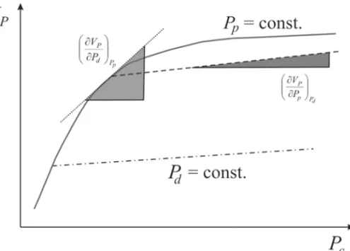
Figura 1– Schematic diagram illustrating how to compute the derivatives on the numerator and denomi-nator in the experimental equation for the effective-stress coefficient (Eq. (6)). The numerator is calculated from the slope of theVP−Pccurve at constantPd, and the denominator is calculated from the slope of
the tangent ofVP−Pcat constantPp. Note thatVPcould be replaced with any rock property.
Besides time-lapse seismic, geopressure prediction on pe-troleum exploration also assumes that the effective stress is equal to the differential pressure. This is a very important issue, since “subsurface geopressures are often the dominant decision varia-ble in the selection of drilling fluids and wellbore casings, which are two of the largest costs in most drilling programs. Under-designing the drilling fluid or casing program can result in un-planned expenses, nonproductive time due to fluid influx, fluid loss or wellbore instability, inability to reach total depth, and even catastrophic environmental damage, blow-outs, or rig fires” (Standifird et al., 2004).
METHOD
It were measured the elastic velocities at ultrasonic frequencies on the laboratory by the pulse transmission technique (Vasquez et al., 2000) on a set of limestone and sandstone samples. The samples were saturated with brine to simulate thein situ
forma-tion water (65000 ppm of NaCl for the limestone and 240000 ppm for the tight sand).
The velocities were measured varying the confining pressure from atmospheric up to 6000 psi. The porepressure was increa-sed until 4000 psi in 500 psi steps. On the other hand in some samples it was used 8000 psi for the final confining pressure.
From the experimental data, it was derived empirical po-repressure coefficients for compressional-wave and shear-wave velocities and also for the bulk and shear moduli. The empirical
coefficients were derived using Equation (5), through the scheme illustrated on Figure 1. Note that a constant differential pressure curve with positive slope corresponds tonless than unity, while those with negative slope correspond ton greater than 1. The case in whichn =1corresponds to a perfect horizontal “Pd =
constant” curves (Vasquez et al., 2007).
In order to obtain the derivatives of velocities and moduli re-lated to a confining pressure, it had been fitted the data points with functions generally used to describe the velocity-pressure beha-vior of rocks, especially the Mavko (2004) and Eberhart-Phillips et al. (1989):
V(P)=aM−bMexp
− P
cM
(8)
and
V(P)=aH +bH −P−cHexp(−dHP) (9)
respectively. Similar pressure laws were used for the bulk and shear moduli. The results obtained with these different pressure laws were very consistent (both fitted functions are shown in fi-gures illustrating velocities and moduli as a function of confining pressure as large and small dashed lines, and they are almost always coincident, as can be seen on those pictures).
corresponding effective-pressure coefficient. The effect of fluid changes was removed using Gassmann’s equation (Gassmann, 1951):
KN
Ksol−KN
= Ksat
Ksol−Ksat
−1
φ
Kf l
Ksol−Kf l
− Kf l N
Ksol−Kf l N
(10)
were KN is the desired normalized bulk modulus,Ksat is the
measured bulk modulus with rock saturated with fluid which bulk modulus is Kf l, andKf l N is the fluid bulk modulus used as
the reference for normalization. It was used the lowest porepres-sure as the reference saturation state. The fluid properties were obtained from the relations published by Batzle & Wang (1992). This approach does not take into account frequency related effects on seismic velocities.
SAMPLE SET
The samples selected for this study comprises unconsolidated to medium consolidated limestones and a set of tight sandstones.
The limestones are calcirudite to rhodolite with a matrix that varies from micritic to calcarenitic. Some samples have also sili-ciclastic grains (mainly quartz). The occurrence of macro-forami-nifera is common as well. Since these limestones were not very well consolidated, the samples were covered with metal jackets with pervious screens at the ends to avoid sample degradation during cleaning as well as petrophysical and acoustic measure-ments. Although this jacketing process had been proved not to change the velocities measurements, in some cases the quality of waveform signal is very poor, especially for the shear wave in saturated samples. Due to these difficulties, it was not possible to pick a complete set of measurements unless on three samples (5005, 5062 and 5070). On the other hand, compressional-wave data collection was possible on six samples. The petrophysical properties of the samples are listed in Table 1. Figure 2 illustra-tes photos from thin sections representing two of the limestone samples and a scanning electron microscopy (SEM) showing the existence of complex micro porosity on these rocks.
Table 1– Petrophysical properties of the limestone samples. Sample ρma(g/cc) φ(%) κ(md)
5001 2.71 23.15 2.25 5005 2.75 29.74 7.63 5057 2.70 33.52 1097.9 5062 2.72 30.78 1237.05 5070 2.67 26.24 34.11 5088 2.71 26.46 225.17
Figure 2– (a) Optical microscopy photo of the limestone sample 5005. This is a calcirudite with calcarenitic matrix, with intergranular porosity. (b) Thin section from sample 5062, biolitite to red algae with vugular porosity. (c) SEM image of sample 5062.
sa-turated samples. The petrophysical properties of the sandstones are listed on Table 2. Note that the porosity of these sandstones is large mainly due to the micro porosity associated to the presence of chlorite. In this sense, it may be considered tight sandstone. Figure 3 shows thin sections images of the sandstone facies, with detail of the fringes as well as a SEM image illustration the grain boundaries.
Table 2– Petrophysical properties of the sandstone samples.
Sample ρma(g/cc) φ(%) κ(md)
5965 2.66 18.50 0.90 5976 2.65 15.20 8.66 6047 2.65 13.20 11.17 6090 2.65 19.40 14.46 6125 2.65 18.00 16.04 6492 2.66 16.50 0.31
RESULTS Carbonates
In Figure 4 it can be observed an example of compressional-wave velocityversusconfining pressure curves for the sample 5005,
with the zero porepressure curves (dots) along with the velocity data for distinct differential pressure values. Actually, zero pore-pressure means atmospheric pore-pressure (14.7 psi or 0.1 MPa). The data for low differential pressure (1000 psi or 6.89 MPa) shows some dispersion around the fitted line. It was also noticed that data for high differential pressure suggestsnvalues higher than unity. In principle the velocity curves for different porepressure values would be “parallel” to each other if the porepressure coef-ficient was equal to unit. From Figure 5, which shows the velocity
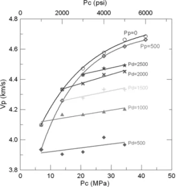
versus confining pressure for different porepressure values for
sample 5005, it becomes evident thatnis not equal to 1. The measurements were repeated successively with different stress paths and in some limestone samples the repeatability was not as good as expected. These “bad results” were associated with sample destruction, maybe due to pressure cycling and cal-cite dissolution. Since calcal-cite is more soluble in brine than in fresh water we could try to avoid this problem using a tampering solution. In some samples there were strong evidences that the dissolution was followed by migration of thin particles and sub-sequent obliteration of the pore space and permeability reduction. From an initial selection of ten samples, four were destroyed by these procedures. Of course, these “bad results” were abando-ned through our study, since the samples lost the integrity during the experiment.
Figure 3– (a) Typical thin section image of the sandstone samples. This is a fine to medium grained sandstones, poorly sorted with disperse large grains. (b) Detail of the grain boundaries with chlorite fringes. (c) SEM image of sample 5965.
pressure curves. It is worth to point out that the normalization of the bulk modulus leads to effective pressure coefficients close to one for moderate and low differential pressure values. This effect was present on the other samples as well: thenvalues corres-ponding to the normalized bulk modulus is equal or very close to unity. In general, for higher differential pressures (and confining pressure)ntends to be greater than unit.
Figure 4– Velocity curves for sample 5005 as a function of confining pressure for zero porepressure (dots) along with constant differential pressure curves.
Figure 5– Velocity curves for sample 5005 as a function of confining pressure for different porepressure values.
Figure 6– Bulk modulus curves for sample 5005 as a function of confining pressure for zero porepressure (dots) along with constant differential pressure curves.
Figure 7– Normalized bulk modulus curves for sample 5005 as a function of confining pressure for atmospheric porepressure (dots) along with constant dif-ferential pressure curves.
are closer to one. Besides, there is a sharp variation onnvalues at 2500 psi and 3000 psi (17.24 and 20.68 MPa, respectively) that needs a better understanding. We suspect that this may be associated with pore space alteration due to brine-calcite interac-tion and pressure cycling or with the presence of bi-modal poro-sity distribution. Pore compressibility experiments on neighbor samples, not shown in this article, also exhibits anomalous beha-vior around these pressures.
Figure 8– Effective pressure coefficients for the bulk modulus of sample 5005 before (diamonds) and after (dots) the normalization process, among with the classical Biot-Willis coefficient for bulk compression of porous material, for at-mospheric porepressure.
Figure 9– Bulk modulus curves for sample 5062 as a function of confining pressure for porepressure vented to the atmosphere (dots) along with constant differential pressure curves.
Figures 9 and 10 show the behavior of the bulk and shear moduli for another limestone sample (5062) for various differen-tial pressures along with the data for the pore system vented to the atmosphere (dots). The data are quite consistent.
Figure 10– Shear modulus curves for sample 5005 as a function of confining pressure for porepressure vented to the atmosphere (dots) along with constant differential pressure curves.
Figure 11– Effective pressure coefficient for the normalized bulk modulus for three limestone samples at 500 psi (3.45 MPa) porepressure. Dashed lines cor-respond to the Biot-Willis coefficient.
data at 4500 psi (31.03 MPa). These data points are listed in Ta-ble 3. Figure 12 summarizes the results of effective pressure co-efficients for the P-wave velocity for all the limestone samples, for a constant porepressure of 500 psi (3.45 MPa). There are some evidences thatndepends on differential pressure.
Table 3– Empirical effective pressure coefficients for the normalized bulk modulus of three limestone samples at 500 psi (3.45 MPa) porepressure.
Pp=500 Effective pressure coefficientn Pc(psi) 5070 5062 5005
1500 0.99 0.99 0.97 2000 1.00 1.01 1.00 2500 0.96 1.02 1.00 3000 0.96 1.00 0.93 3500 1.01 0.99 1.09 4000 1.04 0.99
4500 1.05 0.88 5000 1.09 1.01
Figure 12– Effective pressure coefficients for the compressional-wave velocity of the limestone samples for a constant porepressure of 500 psi (3.45 MPa).
Sandstones
Due to the low permeability of the sandstone samples and the clorithe-brine interaction, that causes obliteration of pore-throats, it was difficult to obtain full water saturation by the imbibition method for all samples. The saturation was then estimated by weighting the sample before and after the saturation process and the fluid bulk modulus used for the calculations were estimated by the Wood’s formula (compressibility equals to the weighted ave-rage of brine and air compressibilities).
The compressional and shear-wave velocity data for the sandstone 5976 (Sw=89%) are illustrated on Figures 13 and 14,
along with the curves for constant porepressures, atmospheric and 500 psi (open dots and open diamonds). The compressional-wave velocity and bulk modulus for sample 5965 at various differential pressures are illustrated on Figures 15 and 16, along with the curve for 500 psi (3.45 MPa) constant porepressure (open dots). The brine saturation for this sample was estimated to be 57%.
Figure 13– Compressional-wave velocity as a function of confining pressure for sandstone sample 5976 for atmospheric and 500 psi porepressure (open dots and open diamonds) along with constant effective pressure curves.
The effective pressure coefficients for compressional-wave velocity for all the sandstones samples are shown on Figure 17 as a function of porepressure for a constant confining pressure 2500 psi (17.24 MPa). As can be noted, it seems that then values depend on porepressure itself. This is another issue on time-lapse studies.
Figure 15– Compressional-wave velocity for sample 5965 at various differen-tial pressures along with the curve for 500 psi (3.45 MPa) constant porepressure (open dots).
Figura 16– Bulk modulus for sample 5965 at various differential pressures along with the curve for 500 psi (3.45 MPa) constant porepressure (open dots).
Figure 17– Effective pressure coefficients for the compressional-wave velo-city for all the sandstones samples as a function of porepressure for a constant confining pressure 2500 psi (17.24 MPa).
It is interesting to compare thencoefficients for the sands-tone and limessands-tone samples. Figure 18 (a) and (b) summarizes thenvalues obtained for the compressional-wave velocity of the sandstones and limestones, respectively, as a function of porosity, for a porepressure of 500 psi (3.45 MPa) and confining pressure of 2500 psi (17.24 MPa). The data points are listed on Table 4. In spite of the data scattering, there is a trend of increasingnwith porosity even considering the different kinds of rock composition and texture.
Table 4– Effective pressure coefficientsnfor the compressional-wave velocity of the sandstone and limestone samples at 2500 psi (17.24 MPa) confining pres-sure and 500 psi (3.45 MPa) poreprespres-sure with the porosityφ(decimal units).
Rock type Sample n φ
Sandstone
6047 0.87 0.1320 5976 0.78 0.1520 6492 0.72 0.1615 6125 0.8 0.1800 5965 0.92 0.1850 6090 0.81 0.1940
Limestone
5001 0.84 0.2315 5070 0.93 0.2624 5088 0.57 0.2646 5005 0.92 0.2974 5062 0.95 0.3078 5058 1.00 0.3352
DISCUSSION
It was found effective pressure coefficientsndifferent than unity, even for the high porosity limestone samples.
The values reported here for the effective pressure coefficient are relatively close to unity when compared to those reported by Xu et al. (2006), that obtainednvalues as low as 0.3 for Lyons sandstone, that is a clean tight sandstone. It must be remembered that our limestone samples are very porous, unconsolidated and that the pore space is well communicated. On the other hand, our sandstone samples are very well consolidated and have relatively low permeability, with much of the porosity contained on shales. This deviation of the effective pressure coefficient from unit can lead to erroneous porepressure interpretation from time-lapse data and even on the feasibility study phase or on geo-pressure prediction. The error due to the n value comes from the fact that, for some porepressure variation1Pp, assuming
a constant confining pressure, the effective pressure variation is 1Pe f = −n1Pp, while the differential pressure variation is
1Pd = −1Pp. As an example, forn =0.8 the variation of
differential pressure is 25% greater than the variation on the
ef-fective pressure. So, for an observed change in the porepressure, we would have an overestimation of changes in bulk modulus. On the other hand, an observed change in seismic velocity or im-pedance would lead to underestimates of the porepressure varia-tion. The error does not depend only on thenvalues, but also on the velocity-pressure sensitivity for the particular reservoir.
Although then values for the unconsolidated limestone are not so far from unity, it has a stronger pressure sensitivity of ve-locities and elastic moduli when compared to consolidated rocks, so that any pressure variation should correspond to a large varia-tion on the elastic property.
Another important issue is that the effective pressure coeffici-ent seems to depend on the porepressure, so that for each time-step on a 4D study, a differentnvalue must be considered.
CONCLUSIONS
We measured the effective pressure coefficients for the seismic velocities and elastic moduli of Brazilian limestones and sandsto-nes. The results show that, even for unconsolidated rocks, there is a deviation of the effective pressure coefficient from unity that can lead to errors on porepressure prediction from seismic data and also on time-lapse studies. These striking results are the first obtained for Brazilian rocks. Nevertheless, more experimental in-vestigations with different rock and fluid types are needed in order to obtain a better understanding of the effective pressure coeffici-ents and its influences on pressure estimation from seismic data.
ACKNOWLEDGEMENTS
The authors thank Petrobras for the permission to present this paper. We are strongly in debt also with the geologists Miguel Pittella Franco and Dorval Dias Filho for the geological des-cription of the samples and useful discussions as well as with Angela Vasquez for revising the manuscript and giving valuable suggestions.
REFERENCES
BATZLE M & WANG Z. 1992. Seismic properties of pore fluids. Geophy-sics, 57: 1396–1408.
BERRYMAN JG. 1992. Effective stress for transport properties of inho-mogeneous porous rock. J. Geophys. Res., 97: 17409–17424.
BERRYMAN JG. 1993. Effective stress rules for pore-fluid transport in rocks containing two minerals. Int. J. Rock Mech. Min. Sci. & Geo-mech. Abst., 30: 1165–1168.
BIOT MA & WILLIS DG. 1957. The elastic coefficients of the theory of consolidation. J. Appl. Mech., ASME, 24: 594–601.
CHRISTENSEN NI & WANG HF. 1985. The influence of pore pressure and confining pressure on dynamic elastic properties of Berea Sand-stone. Geophysics, 50: 207–213.
EBERHART-PHILLIPS D, HAN DH & ZOBACK MD. 1989. Empirical rela-tionships among seismic velocity, effective pressure, porosity, and clay content in sandstone. Geophysics, 54: 82–89.
GASSMANN F. 1951. On Elasticity of Porous Media. In: PELISSIER MA, HOEBER H, COEVERING N & JONES IF (Eds.). Classics of Elastic Wave Theory. SEG Geophysics Reprint Series No. 24, SEG, 389–407.
GUREVICH B. 2004. A simple derivation of the effective stress coefficient for seismic velocities in porous rocks. Geophysics, 69: 393–397.
KING MS. 1966. Wave velocities in rocks as a function of overburden pressure and pore fluid saturants. Geophysics, 31: 56–73.
LADE PV & DE BOER R. 1997. The concept of effective stress for soil, concrete and rock. G´eotechnique, 47: 61–78.
MAVKO G. 2004. Seismic Fluid Detection, Reservoir Delineation, and Recovery Monitoring: The Rock Physics Basis. Course presented at the 74thSEG Meeting, October 9-10, Denver, Colorado. 327 pp.
NUR A & BYERLEE JD. 1971. An exact effective stress law for elastic deformation of rocks with fluids. J. Geophys. Res., 76: 6414–6419.
PRASAD M & MANGHNANI M. 1997. Effects of pore and differential
pressure on compression wave velocity and quality factor in Berea and Michigan sandstones. Geophysics, 62: 1163–1176.
SKEMPTON AW. 1960. Significance of Terzaghi’s concept of effective stress. In: TERZAGHI K (Ed.). From Theory to Practice in Soil Mecha-nics. John Wiley & Sons Inc. 425 pp.
STANDIFIRD W, MATTHEWS M & PAINE K. 2004. Optimized basin mo-deling for geopressures. Petroleum Africa, December 2004: 6–10.
TERZAGHI K, PECK RB & MESRI G. 1996. Soil Mechanics in Engine-ering Practice, 3rdedition. John Wiley & Sons Inc. 592 pp.
TODD T & SIMMONS G. 1972. Effect of pore pressure on the velocity of compression waves in low-porosity rocks. J. Geophys. Res., 77: 3731–3743.
VASQUEZ GF, SIM ˜OES FILHO IA, BRUHN CHL & DILLON LD. 2000. Viscoelastic behavior of a Brazilian turbidite reservoir and its relati-onships to facies attributes. In: 70thAnnual International Meeting. SEG.
Expanded Abstracts: 1927–1930.
VASQUEZ GF, VARGAS E, LE˜AO M, BACELAR C, JUSTEN J & ALVES I. 2007. Effective pressure coefficients of some Brazilian rocks. In: Tenth International Congress of the Brazilian Geophysical Society. November 19-23, Rio de Janeiro, Brazil. CD-ROM.
XU X, HOFMANN R, BATZLE M & TSHERING T. 2006. Influence of pore pressure on velocity in low-porosity sandstone: Implications for time-lapse feasibility and pore-pressure study. Geophys. Prospect., 54: 565–573.
NOTES ABOUT THE AUTHORS
Guilherme Fernandes Vasquezholds a BSc in Physics from Universidade Federal do Rio de Janeiro (UFRJ, 1988) and a MSc in Reservoir Engineering from Universidade Estadual de Campinas (UNICAMP, 1999). He joined Petrobras in 1989 and currently works at the Petrobras’ Research Centre in Geophysics, acting in research projects and technical support. He develops studies especially on rock physics, rock-log-seismic calibration, time-lapse seismic and geomechanics’ effects on rock velocities. Some of these studies are being conducted in collaboration with the researchers from the Geology Department of Federal University of Rio de Janeiro.
Eur´ıpedes do Amaral Vargas Juniorholds a BSc in Civil Engineering from Universidade de S˜ao Paulo (USP, 1972), and a MSc in Geotechnical Engineering from Pont´ıficia Universidade Cat´olica do Rio de Janeiro (PUC-Rio, 1975) as well as MSc and PhD in Rock Mechanics from the Imperial College, University of London (1978 and 1988, respectively). He is currently professor at the Departamento de Engenharia Civil from Pont´ıficia Universidade Cat´olica do Rio de Janeiro and at the Geology Department of Federal University of Rio de Janeiro, where he is working developing research studies on Environmental Geotechnics, Petroleum Geomechanics and Rock Mechanics.
Cleide Jeane Bacelar Ribeiroholds a BSc in Civil Engineering from Universidade Estadual de Feira de Santana (UEFS, 1996) and a MSc as well as a PhD in Civil Engineering from Pontif´ıcia Universidade Cat´olica do Rio de Janeiro (PUC-Rio, 1999 and 2003, respectively). Former engineering professor in Universidade Federal Fluminense, she joined the Petrobras rock physics team in 2004.
Marcos de Le˜ao Silvahas background in electronics and had worked several years at Petrobras’ seismic crews. He joined the rock physics laboratory staff in 1991 and acts in research studies as well as on lab equipment development.