www.scielo.br/rbg
VARYING PATTERNS OF WATER CIRCULATION IN CANAL DE COTEGIPE,
BA´IA DE TODOS OS SANTOS
Marcelo Augusto Greve Pereira
1and Guilherme Camargo Lessa
2Recebido em 15 fevereiro, 2008 / Aceito em 8 janeiro, 2009 Received on February 15, 2008 / Accepted on January 8, 2009
ABSTRACT.The Canal de Cotegipe is a 30 m deep, 4 km long tidal channel in northeastern Brazil connecting the small Ba´ıa de Aratu (24.5 km2) to the much larger Ba´ıa de Todos os Santos (1223 km2). Several industrial and port facilities surround the channel and Ba´ıa de Aratu, and polluted riverine discharge as well as a direct release of toxic residuals by harbor operations makes the area one of the four polluted hot-spots within Ba´ıa de Todos os Santos. An analysis of current measurements, tidal elevation records and water quality monitoring has allowed for a preliminary understanding of the driving forces that affect the channel. Tidal flows are modulated by the extent of intertidal inundation in the channel and the bay, with stronger ebb-dominant flow conditions associated with neap tides at the seaward end of the channel and with spring tides at the landward end of the channel. Subtidal flows are mainly driven by density gradients normally oriented towards Ba´ıa de Todos os Santos, leading to a vertically stratified, estuarine like flow. This structure is strengthen in the wet season and weakened in the dry season when unstratified or even and inverse estuarine stratification may develop as a result of higher evaporation rates.
Keywords: Ba´ıa de Todos os Santos, estuary, subtidal circulation, Ba´ıa de Aratu.
RESUMO.O Canal de Cotegipe com 30 m de profundidade e 4 km de extens˜ao estabelece a conex˜ao entre a Ba´ıa de Aratu (24,5 km2) e a Ba´ıa de Todos os Santos (1223 km2). Ao redor da Ba´ıa de Aratu e ao longo do Canal de Cotegipe existe uma expressiva concentrac¸˜ao industrial e portu´aria, acarretando em descargas t´oxicas que transformam a regi˜ao em um dos quatro importantes focos de poluic¸˜ao dentro da Ba´ıa de Todos os Santos. An´alises de dados correntom´etricos, maregr´aficos e de qualidade de ´agua permitiram uma avaliac¸˜ao inicial dos mecanismos de circulac¸˜ao ao longo do canal. Os dados indicam que os fluxos de mar´e s˜ao modulados pela extens˜ao de inundac¸˜ao da regi˜ao intermar´es. Uma amplificac¸˜ao do dom´ınio do fluxo de vazante ocorre nas mar´es de quadratura junto `a sa´ıda do canal, e em siz´ıgia na sua extremidade interna. Fluxos com freq¨uˆencia submareal estabelecem-se principalmente devido ao gradiente de densidade normalmente orientado em direc¸˜ao `a Ba´ıa de Todos os Santos, acarretando em uma estratificac¸˜ao vertical de caracter´ıstica estuarina. Esta estrutura de fluxo ´e reforc¸ada no inverno e atenuada no ver˜ao, quando a reduc¸˜ao do gradiente de densidade permite o estabelecimento de fluxos n˜ao estratificados ou at´e mesmo com estratificac¸˜ao estuarina inversa ocasionada pelo aumento das taxas de evaporac¸˜ao.
Palavras-chave: Ba´ıa de Todos os Santos, estu´ario, circulac¸˜ao subtidal, Ba´ıa de Aratu.
1Curso de Graduac¸˜ao em Oceanografia, Universidade Federal da Bahia, Instituto de Geociˆencias, 40170-280 Salvador, BA, Brazil. Present address: Petrobras, E&P-Serv-US-Sub, Rodovia Amaral Peixoto, 27925-290 Maca´e, RJ, Brazil. Phone: +55(22) 2761-5431 – E-mail: [email protected]
INTRODUCTION
Exchange flows in estuarine zones are driven by two main process called tidal pumping/trapping and steady baroclinic flows (Martin et al., 2007). The former acts at tidal frequencies and is associ-ated with the spatial characteristics of the flow (jet or radial flow) and with differences in phase of the cross-section averaged tidal velocity and scalar concentrations. The latter acts at subtidal fre-quencies and are associated with density gradients that induce stratified flows. Flow stratification coupled with vertical gradients of a scalar in the water column will lead to exchanges between dif-ferent sectors of the estuary or between the estuary and the ocean. Because estuarine flows are influenced by freshwater runoff, atmospheric water balance, winds and tidal and subtidal sea-level oscillations the circulation driving mechanisms for both tidal and subtidal frequencies may change seasonally. Therefore, retention or importation of suspended matter and solutes may alternate with periods of exportation at given times of the year or at some tidal conditions (Stacey et al., 2001).
The Canal de Cotegipe is a 30 m deep, 4 km long tidal channel in northeastern Brazil connecting small Ba´ıa de Aratu (24.5 km2)
to the much larger Ba´ıa de Todos os Santos (BTS) (1223 km2)
(Fig. 1). One hundred and seventy different industries including textiles, mechanics, agricultural, siderurgical and petro- and che-mical unities have been installed at the vicinities of Ba´ıa de Aratu in the last 60 years (CRA, 2004). Also, a large State-owned commodity port (Aratu) and three private ports (Navy, Ford and Moinho Dias Branco) are located along Canal de Cotegipe. This intense industrial occupation gives rise to polluted riverine dis-charge as well as a direct release of toxic residuals due to har-bor operations making the area one of the four polluted hot-spots within the BTS. The clayey sediment size inside the bay have favored the retention of pollutants such as lead, copper and zinc, adhered both to suspended and bottom sediments (Freire Filho, 1979; Alves, 2002; CRA, 2004).
This paper analyses existing sets of hydrodynamic and water quality data collected along Canal de Cotegipe in different years covering the annual seasonality of the area. The study aims to contribute with the understanding of the flow structure in the channel and the potential for scalars’ exchange between the Ba´ıa de Aratu and BTS.
STUDY SITE
Ba´ıa de Aratu is a small system that includes the bay itself and a 4 km long channel (Canal de Cotegipe) that connects the central part of the bay to the BTS. Ba´ıa de Aratu is centered at 12◦47.1′S
and 38◦28.2′ W, with a maximum width and length of 214 m and 4.1 km, respectively. The bay is shallow (Fig. 1), with an area weighted depth of 1.8 m and intertidal depths that account for 24% (5.7 km2) of the whole bay area. Eighty five percent
the bay is shallower than 5 m, and areas deeper than 10 m are basically restricted to Canal de Cotegipe, where a maximum of 40 m is recorded.
The climate in the region is tropical humid, with an an-nual mean temperature, precipitation and evaporation of 25.3◦C, 2086 mm and 1002 mm, respectively (Salvador Meteorological Station – INMET, 1992). Two well defined, wet and dry sea-sons exist. The wet season spans from March to July (Fig. 2), when it rains 60% of the total annual precipitation. The maxi-mum monthly average (1930-1990) precipitation is 322 mm in May, whereas the minimum is 90 mm in January. The dry se-ason spans from August to February, with a period of slightly higher precipitation in November. Mean annual evaporation amounts to 96 mm, with monthly rates varying between 80 mm (May) and 110 mm (January). The fluvial discharge from a small catchment area reaches the bay via two perennial rivers, Santa Maria and Cotegipe Rivers, which together have an estimated average annual discharge of 1.65 m3s–1(CRA, 2000).
Precipitation and evaporation rates are similar during the dry season. The atmospheric water balance, which is net positive an-nually, can be negative during the dry season as it is shown in the climatology for the years 1931-1960 (Fig. 2b). Monthly mean temperature variation throughout the year is approximately 3◦C (INMET, 1992), with maximum mean values between January and March (26,7◦C) and minimum between July and August (24◦C). The tides in the BTS are characteristically semi-diurnal, and ranges increase up bay by a factor of 1.5 (Cirano & Lessa, 2007). M2 amplitude grows from 0.67 m in the ocean to 0.89 m in
the center of the bay and 1.06 m in the westernmost bay reach. A tide gauge deployed for 39 days in 1988 at the entrance of Canal de Cotegipe indicates an average spring tide range of 2.31 m (Lessa et al., 2001). Assuming that these ranges are re-produced throughout the bay (with an area of 24.5 km2), the
ti-dal prism is about 5.3×10⁶m3. Given the annual mean fresh
water discharge of 1.65 m3s–1 (CRA, 2000), hence the
fresh-water inflow during a full tidal cycle corresponds to less than 1% of the spring tidal prism.
The wind field shows strong seasonality, blowing from E and SE in the dry season and from S and SW in the wet season. Ave-rage and maximum wind magnitude at Ilha dos Frades (Fig. 1), in the center of the BTS, is about 5 m s–1and 12 m s–1
Figure 1– Location and bathymetry of Canal de Cotegipe and Ba´ıa de Aratu, with the location of instrument sites. Cir-cles identify current and water-quality stations, whereas triangle indicates the tide gauging station. Vertical datum is the hydrographic datum, normally 1.45 m below mean sea level.
Jan Feb Mar Apr May Jun Jul Aug Sep Oct Nov Dec -100
0 100 200 300
1931-1960 1961-1990
Jan Feb Mar Apr May Jun Jul Aug Sep Oct Nov Dec 50
100 150 200 250 300 350
(m
m
)
Precipitation Evaporation
not exert significant influence on its circulation, as indicated by Cirano & Lessa (2007).
DATA SET
Tides
The tide was monitored between April 2006 and January 2007 with a digital pressure sensor Global Logger installed at the Aratu Navy Base (Fig. 1). The pressure sensor was fixed inside a PVC tube and the logger was configured to get a single reading every 3 minutes. Although the data was downloaded regularly (about every two weeks), battery failure and instrument malfunction caused several data losses.
Harmonic analysis of the longest data set (112 continuous days between July and November 2006), was performed accor-ding to Franco (1988) with the aid of the software PacMare. This same data set was used to determine the tidal ranges and tidal asymmetry, as well as the power spectral density with the Fast Fourier Transform. A Fourier low-pass filter, with a cut off period of 73 hours (equivalent to a Doodson filter), was used to separate low frequency fluctuations from the tidal oscillations throughout the time series.
Tidal distortion or asymmetry was calculated by the ratio of rising over falling tide time(LogeRt/Ft). The natural logarithm
of this ratio instead of the ratio itself was used in order to provide an equal distribution of both positive and negative asymmetries in relation to a symmetrical tidal form(LogeRt/Ft = 1).
Ne-gative (positive) ratios indicate that the falling (rising) tide lasts longer than the rising (falling) tide.
Currents
Long-term records of the current speed and direction were ob-tained by means of moored ADCP’s and Aanderaa’s RCM-7 cur-rent meters. Moored ADCP data was provided by the National Oceanographic Data Bank (BNDO), whereas moored RCM-7 and S4 records were published by CRA (2000). The current vectors were decomposed in along-channel and cross-channel compo-nents, with positive values associated with the westward (ebb) flow in the former and southward flow in the latter. Negative along-channel velocities were flood directed.
Fourier low and high pass filters were used to separate su-pratidal and low frequency current fluctuations in all time series. Respective cut off periods were 53 hours (corresponding to the inertial period at this latitude) and 12.4 hours (tidal frequency). In order to investigate tidal current asymmetry, maximum ebb and maximum flood current speeds for each tidal cycle were
ex-tracted from the supratidal time series. Again, the natural loga-rithm of the ratio between maximum flood and maximum ebb current speed were calculated. Astronomical tidal constituents were calculated according to Franco (1988) with the aid of the software PacMare.
Moored ADCP’s
Two RDI ADCP Sentinel 300 kHz were moored (stations #101 and #201 in Fig. 1) at the bottom of Canal de Cotegipe from November 12 to December 14 2002 (dry season) and from June 14 to July 16 2003 (wet season) at water depths of about 25 m. Equipment malfunction stopped data acquisition after 3 weeks after being deployed in the dry season. Velocity data was obtained every 1 m starting at 3 m above the bottom up to the surface. Mea-surements close to the surface were affected by reflection, and the identification of biased measurement depths was performed by comparing the standard deviation of the current magnitudes. In both stations valid data extended up to 2 m below the lowest low tide during the campaign. Mean velocity magnitude and direction was calculated after a 1 minute burst (at 2 Hz) every 15 minutes. The water surface refers to the lowest low tide during the campaign.
Moored RCM-7 and S4
Two RCM-7 were moored at station #3 (Fig. 1) at depths of 8.7 m and 24.3 m. The instruments recorded synchronously every 0.25 hour for 15 days, between January 10 and January 25, 1999 (dry season) and between May 22 and June 6, 1999 (wet season).
Water properties
Time series of water temperature, conductivity and density were recorded with Seabird CTD’s and published by CRA (2000) for two field campaigns coincident with the RCM-7 moorings. The measurements took place at stations #3 (Canal de Cotegipe) and #16 (BTS) (Fig. 1), both in the dry and wet seasons during a spring (January 18 and May 29, 1999) and neap (January 24 and June 06, 1999) tide.
RESULTS Tides
Tides in Canal de Cotegipe are semi-diurnal, with form number
respectively (Table 1), indicating an amplification of 0.11 m and a delay of about 12◦in relation to the tide at the entrance of BTS (Cirano & Lessa, 2007). The mean tide range was 1.88 m, whe-reas the maximum reached 3.33 m close to the equinox in Sep-tember (Fig. 3). This range is 0.5 m larger than the maximum previously recorded in the same location by the Brazilian Hydro-graphic Authority (Lessa et al., 2001).
Table 1– Harmonic constituents of the tide at Canal de Cote-gipe (see Fig. 1 for station location). Phase is relative to GMT.
Constituent Amplitude Phase (cm) (◦)
O1 6.84 125.16
K1 4.27 208.37
Q1 2.37 97.2
P1 1.15 192.76
M2 90.93 114.07
S2 30.37 127.87
N2 17.26 110.28
K2 9.75 126.82
L2 6.54 82.44
MU2 4.06 132.91
M4 1.98 299.09
MS4 1.81 21.97
29 12 26 9 23 7 21 4 -50 0 50 100 150 200 250 300 350
Aug Sep Oct Nov 2006 E le va ti o n ( cm )
Figure 3– Tidal record and the low–pass filtered signal (in white) in Canal de Cotegipe.
Variance analysis of the reconstituted and measured tides shows that the astronomical signal is responsible for 98% of the observed changes in the sea surface elevation. Subtidal oscil-lations varied in height between 0.10 m and 0.17 m (Fig. 3), with periods ranging from 9 to 13 days in accordance with the spectral signature of the time series (Fig. 4). The energy con-centration at 27 days is ascribed to differences between consecu-tive spring tides in the analyzed record, which included a lunar perigee/apogee cycle.
Frequency (cycles per hour)
P o w e r D e n s it y ( c m ²) 12.4 hours 24.8 hours
13 days 7 days 5 days 27 days
Figure 4– Spectral signature of the tidal series.
Overall, tidal distortion in Canal de Cotegipe causes a shor-ter falling tide. The average and maximum duration of the rising tide in the whole data set is 6.4 hours and 7.5 hours, respecti-vely. Figure 5 shows the plot of the natural logarithm of the ratio between the duration of the rising and falling tide for each tidal cycle against its respective high tide level. The data distribution shows that the large majority of the ratios are positive (shorter falling tides), with larger ratios, or more distorted tides, occur-ring duoccur-ring neap tides. The fewer negative ratios become less numerous at larger tide ranges, where the tides tend to a symme-trical form.
ADCP current measurements
The mean vertical current velocity magnitude in Canal de Cote-gipe was around 0.17 m s–1, with maximum velocity magnitudes
of 0.49 m s–1in the landward end of the channel (stations #101
and #3 – Fig. 1) and 0,70 m s–1 at the seaward end (#201 –
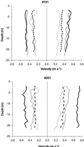
Fig. 1). The along channel current component was five to seven times stronger than the cross channel component, especially at stations #101 and #3. The vertical variation of maximum velo-city of the longitudinal component during spring and neap ti-des is shown in Figure 7 for the both dry season. It is obser-ved that maximum current velocities were associated with the ebbing tide at both stations, reaching 0.54 m s–1at station #101
and 0.75 m s–1at station #201. Maximum current velocities at
neap tides were about half that during springs.
0.4 0.6 0.8 1 1.2 1.4 1.6 1.8 -0.4
-0.3 -0.2 -0.1 0 0.1 0.2 0.3 0.4
Predicted high tide level (m)
ln
(∆ t flo
o
d
/∆ t e
b
b
)
Figure 5– Variation of the tidal asymmetry (ratio of the rising and falling tide duration) with the high tide level at the respective tidal cycle. A ratio of 0.69 (–0.69) indicates that the rising (falling) tide is twice as long as the falling (rising) tide. The thick line represents the linear best fit on the data set.
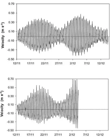
Figure 7– Variation of the depth averaged longitudinal component of the current velocity at stations #101 (upper) and #201 (lower) during the dry season of 2002. Positive (negative) values are ebb (flood) directed.
ebb (flood) dominance in the dry season occurred during neap (spring) tides. In the wet season the log ratios are rather scatte-red, and a clear trend is indiscernible.
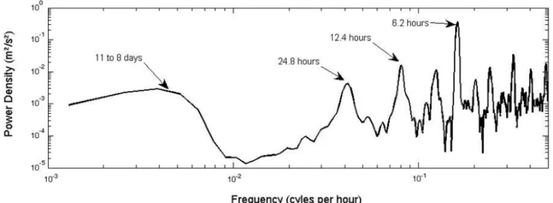
Variance analysis of the reconstituted tidal current field after harmonic analysis shows that the astronomical tides explained between 91% (surface) and 98% (bottom) of the current variance at station #101, and between 75% (surface) and 93% (bottom) of the same variance at station #201. The most important tidal current components are M2, S2 and N2, which account for 37%, 16%, and 6% of the total tidal energy. Subtidal circulation, ac-countable for some of the remaining current variance, had fre-quencies of 8 to 11 days (Fig. 9) as suggested by the energy density distribution at station #101.
The magnitude of the low-pass filtered currents (Fig. 10) were about 10% of the tidal currents, with the exception of the ebb-oriented surface flow that attained up to 0.21 m s–1at station
#101 (dry season) and 0.13 m s–1at station #201 (dry and wet
seasons). It is observed that the current direction changes along the water column, ebbing at the surface and flooding at the bot-tom, as a classic gravitational estuarine circulation. In fact, the computed residual currents (Fig. 11) indicate the existence of a classical estuarine circulation at both stations either in the dry and in the wet seasons. Residual current magnitude varied between 0.02 m s–1and 0.03 m s–1. A stronger gravitational circulation
occurred in the wet season, when rainfall is higher.
Other modes of circulation are also indicated in Figure 10. It is noticed that there were occasions when unidirectional out-going flows (station #201 in the dry season around days 8 and 20), unidirectional incoming flows (station #101 in the wet sea-son around day 12) and even a short-lived inverse estuarine gra-vitational circulation (station #101 in the dry season around day 27) were established.
Anchored Aanderaas
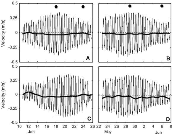
Currents measured at station #3 in 1999 had similar magnitu-des to those recorded in 2003 at the neighboring station #101. Figure 12 shows the variation of the longitudinal current com-ponent. Averaged and maximum magnitudes for the upper and lower instruments were approximately 0.17 m s–1and 0.41 m s–1,
Figure 8– Variation of the predicted high water elevation and the natural log ratio of the maximum flood and maximum ebb current velocity for different depths in the water column. Thick line indicates the mean ratio for the water column. For reference, a ratio of 0.69 (–0.69) means that the flooding (ebbing) tide is twice as fast as the ebbing (flooding) tide.
The maximum subinertial current magnitude was recorded in the wet season, equaling 0.08 m s–1at the bottom (Fig. 12).
Landward-directed flow prevailed in the two stations both in both dry and wet seasons. A worth noting exception occurred in the beginning of the dry season record when an inverse estuarine circulation was shortly established. The residual currents had an average value of -0.02 m s–1at all stations.
Low frequency oscillations with periods of 2-3 days were recorded in the wet season in both (surface and bottom) cur-rent meters, being partially in phase. The correlation between
the surface and bottom filtered time series was high in the dry season (R2 = 0.81), but non-existent in the wet season
(R2= 0.09).
Water Properties
Figure 9– Energy density distribution of the current velocity time series (#101) in the dry season.
above 28◦C. This thermohaline characteristics indicates that the tropical water (TW) mass is advected into Ba´ıa de Todos os Santos in the dry season, as reported by Cirano & Lessa (2007). Maxi-mum values of temperature and salinity were recorded on Febru-ary 2006, reaching 30.5◦C and 37.7, respectively. In the wet sea-son a coastal water mass (CW) was formed, with salinities smaller than 35 and temperatures below 28◦C. Larger temperature vari-ations occurred in the dry season (1.5◦C and 1.3◦C for stations #3 and #16, respectively), whereas salinity differences became more pronounced in the wet season (2.5 and 1.5 for stations #3 and #16, respectively – Fig. 14).
Water temperature was slightly higher inside Ba´ıa de Aratu, where a maximum of 30.5◦C was recorded. Dry and wet sea-sons mean values at station #3 (29.4◦C and 26.9◦C) were about 0.5◦C higher than the respective ones at station #16 (28.7◦C and 26.6◦C). Negligible differences were observed between spring and neap tides (Figs. 15 and 16), and stronger vertical gradients (maximum difference of 0.5◦C between surface and bottom) occurred during the dry season.
Opposite to temperature, the salinity gradient inverted from dry to wet season. Salinity values in the dry season were higher at station #3 than at station #16. Mean values at those stations were 37.1 and 36.8, respectively. Salinity at the bottom of sta-tion #16 showed consistent lower values, both in the dry and in the wet seasons regardless of the tidal cycle. This phenomenon may be ascribed to local discharge of an aquifer, possibly along a fault line.
In the wet season, salinity decreased at station #3 in respect to that at station #16 with mean values of 33.8 and 34.5 for those respective stations (Figs. 15 and 16). If the deepest records at station #16 are not taken into account, the vertical salinity
gradi-ent was small at all monitoring campaigns, but smaller during the wet season. Highest vertical gradients were observed in the wet season, with a maximum of 1.3 at station #3.
The density distribution in Figures 15 and 16 shows that the mean density at station #16 was always larger than at station #3, although rather less significant in the dry season. Mean den-sity values at these respective stations were 1023.57 kg/m3and
1023,53 kg/m3in the dry, and 1022.51 kg/m3and 1021.90 kg/m3
in the wet season. The horizontal density gradients were small and with negligible differences between spring and neap tides, but the wet season gradients were two times larger than du-ring the dry season, with means of 0,6×10⁻⁵kg.m–3.m–1and
1.5×10⁻⁵kg.m–3.m–1, respectively. Mean density differences
between the two stations in the dry season were smaller than the standard deviations, suggesting that inversions in the direction of the density gradient may eventually take place.
DISCUSSION
Tidal distortion in Canal de Cotegipe (max1tf lood/1tebb =
1.34) is larger than that verified outside in the center of the BTS (max1tf lood/1tebb =1.03, Cirano & Lessa, 2007), which
can be ascribed to a higher degree of friction imposed on the tidal wave inside the channel. The recorded rising to falling time ratios increased from spring to neap tides as a result of different rates of flooding and the depth distribution within the channel and bay intertidal area. Larger distortion during neap ti-des may be credited to a slow flooding rate of relative ample and low intertidal areas.
Figure 10– Low-pass filtered current field in the water column for stations #101 and #201 in the dry season (upper panels) and the wet season (lower panels).Zis the local depth whereasHis the deepest measured depth (23 m).
Aubrey & Friedrichs, 1988). Ebb-tidal current dominance, how-ever, was not observed throughout the lunar cycle, and took place at contrasting tidal conditions at stations #101 and #201. In the former, closer to the bay, the flow was ebb dominated only during spring tides, whereas at station #201 ebb dominance was recorded at neap tides. Such contrast is likely due to the impact of the estuary hypsometry at the immediate vicinity to the station. Friedrichs & Aubrey (1988) and Lessa (2000) indicate that ebb dominance is proportional to the relative extent of the mangrove area, which in turn depends on the longitudinal position within the estuary. Therefore, the flow at station #101 is more affec-ted by the hypsometry of Ba´ıa de Aratu than station #201, more
influenced by changes in the surface area of Canal de Cotegipe during a tidal cycle. In fact, tidal current asymmetries at station #201 in the dry season reflected the asymmetry ratios of the tidal wave measured by the tide gauge, located a few hundred meters away (Fig. 1). More distorted neap tides caused the expected ebb dominance of the flow. The discrepancies of the tidal cur-rent asymmetry between both stations suggest that tidal wave distortion inside Ba´ıa de Aratu has a different cause from that at the entrance of Canal de Cotegipe, which may be due to a higher elevation of the intertidal areas.
Figure 11– Residual current velocity in the water column at stations #101 and #210 in the dry (thick line) and wet (thin line) seasons. Positive (negative) values are ebb (flood) directed.
role in the tidal oscillations. Subtidal oscillations in Canal de Cotegipe were smaller than 0.17 m, in agreement with the 0.2 m maximum oscillations reported by Lessa et al. (2001) from a 1-year tidal record at Salvador Harbor. The energy distribution within subtidal frequencies shows a peak at 13 days, which is also concurrent to that observed in Salvador harbor (Lessa et al., 2001).
Similarly to water level, currents in Canal de Cotegipe were closely related to the astronomical tides. The correlation and va-riance explanation between observed and predicted tidal currents average 0.88 and 91%, respectively. Cirano & Lessa (2007) re-ported correlation values of 0.90 and variance explanation equal to 85% in the central part of the BTS and observe that wind driven circulation is only significant outside the bay. Therefore, subti-dal circulation in the BTS, as well as in the Canal de Cotegipe, is most likely due to density gradients, low-frequency barotropic circulation and tidal pumping.
Although the water column is apparently well mixed through-out the year, spatial density differences are significant in dri-ving subtidal flows that can exchange water, solids and solutes
between Ba´ıa de Aratu and the BTS. The average density gradient between stations #16 (BTS) and #3 (Canal de Cotegipe) is direc-ted towards the BTS, and increases from 0.6×10⁻⁵kg m–4in
the dry season to 15×10–5kg m–4in the wet season. This
gra-dient is almost twice as large as that verified by Cirano & Lessa (2007) (7.94×10⁻⁵kg m–4) along the main axis of BTS for the
same wet season.
The dry and wet season potential current established by the density gradient between Ba´ıa de Aratu and the BTS was calcula-ted for neap and spring tides by applying the distribution of the time averaged density at equal non-dimensional intervals of the water column. According to Holloway et al. (1992), the magnitude of the density driven currentUcan be assessed by the equation
U(z)= g H 3
ρoKZ δp δx
× (
3
16
1+4a
1+3a
"
Z H
2
−1−2a
# +
1
6
Z H
3 +
1
6+
a
2
)
where Z =elevation (non-dimensional), H =total depth,
-0.5 -0.25 0 0.25 0.5
V
e
lo
c
it
y
(m
/s
)
10 12 14 16 18 20 22 24 26 -0.5
-0.25 0 0.25 0.5
V
e
lo
c
it
y
(m
/s
)
22 24 26 28 30 2 4 6 8
Jan May Jun
Figure 12– Variation of the mean and low-passed (thick line) longitudinal component of the mean current at station #3. A and C are respectively upper and lower current meters in the dry season, while B and D are respectively upper and lower current meters in the wet season. Circles indicate the days of water quality profiling.
to be constant anda =(Kz/k H), wherekis a linear
bottom-friction coefficient given byk =uC0.5
d . The vertical eddy
vis-cosity is estimated by Kz =0.06u∗H, whereas the friction velocity in the water is calculated by u∗ = (ku−H)0.5. The
–Hindex refers touatz= H. Typical values forH,u,u−H
andCdin the Canal de Cotegipe are 30 m, 0.18 m s–1, 0.1 m s–1
and 0.0025, respectively. The equation assumes a steady balance between the horizontal pressure gradient imposed by the density gradient and vertical friction, presuming that the path between both stations is a long narrow channel (Holloway et al., 1992). The vertical distribution for the calculated mean density currents are shown in Figure 17. Current magnitudes are similar to those observed in the wet season, achieving approximately 0.055 m s–1
at the corresponding elevation of the lower current meter. The calculated dry season velocities are however smaller than those observed, and suggest a strengthening of surface flows towards Ba´ıa de Aratu with no stratification. It is possible that other driving mechanism, such as lateral flow variability, was interfering with the low frequency current field at the monitoring site. It is worth noting that the zero-velocity contour occurs between the depths of 0.3 and 0.4, which is about or just above the relative elevation of the upper current meter. This helps to explain the predominance of landward-directed subtidal flows in both current time series.
Density gradient occasionally inverts in the dry season when salinity is increased due to more intense evaporation, overcoming the concurrent rise in the water temperature. Inverse estuarine circulation characterized by subtidal flows exiting Ba´ıa de Aratu through the bottom of Canal de Cotegipe was recorded in the dry season of 2002. Unfortunately, there were no concomitant mea-surements of water quality in- and outside Canal de Cotegipe to verify the density gradient. Moreover, a time series of precipita-tion and evaporaprecipita-tion was not available to investigate the climato-logic thresholds that triggered eventual inversions of the density gradient.
Figure 13– Variation of the natural log ratio between the maximum flood and maximum ebb current velocity against predicted high tide elevation at Canal de Cotegipe. Dry season is in the upper panel and wet season in the lower panel. The lines represent the best linear fit for each station. For reference a ratio of 0.69 (–0.69) means flooding (ebbing) tide is twice as fast as the ebbing (flooding) tide.
Exchange of scalars between Ba´ıa de Aratu and BTS may oc-cur both under unstratified and stratified subtidal flows. In the former, exchange can be driven by tidal trapping, where residual transport of any scalar is created by the difference in phase of the cross-section averaged tidal velocity and the scalar concen-tration. This is especially the case given that asymmetries do exist between ebb and flood currents, what would be expected to cause both exportation and importation of scalars. In the case of strati-fied subtidal flow, which apparently prevails in Canal de Cote-gipe, net material transport will largely depend on the vertical distribution of its concentration. Assuming that scalar concen-trations are homogeneous or even that a gradient exists towards the bottom, landward transport close to the bottom and net-seaward transport close to the surface would exist. In fact Poggio et al. (2005) calculated the suspended sediment transport at the thalweg in the mid-section of Canal de Cotegipe based on the
vertical turbidity field obtained from ADCP observations. The results showed a net-sediment import in the lower 60% of the water column and net export in the upper 40%, with depth avera-ged net import of order of 10–4kg s–1m–1.
Salinity (psu) T e m p e ra tu re (° C ) 19.5 20.7 21.8 23 24.1
31 32 33 34 35 36 37 38 26 26.5 27 27.5 28 28.5 29 29.5 30 30.5 31
Figure 14– Temperature and salinity pairs from CTD measurements at stations #3 and #16 (1999). Dry (wet) season clusters in the upper (lower) right (left) corner of the diagram.δtfields in kg m–3.
0 0.1 0.2 0.3 0.4 0.5 0.6 0.7 0.8 0.9 1
26 26.5 27 27.5 28 28.5 29 29.5 30 30.5
D e p th ( Z ) Temperature (C°) Temperature 0 0.1 0.2 0.3 0.4 0.5 0.6 0.7 0.8 0.9 1
32 33 34 35 36 37 38
D e p th ( Z ) Salinity Salinity 0 0.1 0.2 0.3 0.4 0.5 0.6 0.7 0.8 0.9 1
1021 1021.5 1022 1022.5 1023 1023.5 1024
D e p th ( Z ) Density Density
0
0.1
0.2
0.3
0.4
0.5
0.6
0.7
0.8
0.9
1
26 26.5 27 27.5 28 28.5 29 29.5 30 30.5
D
e
p
th
(
Z
)
Temperature (C°)
0
0.1
0.2
0.3
0.4
0.5
0.6
0.7
0.8
0.9
1
32 33 34 35 36 37 38
D
e
p
th
(
Z
)
Salinity Salinity
0
0.1
0.2
0.3
0.4
0.5
0.6
0.7
0.8
0.9
1
1020.5 1021 1021.5 1022 1022.5 1023 1023.5 1024
D
e
p
th
(
Z
)
Density Density
Figure 16– Mean values of temperature, salinity and density at equal, non-dimensional, intervals of the water column during springttides at stations #16 (dashed line) and #3 (continuous line). Thicker lines (solid and dashed) represent the dry season and thinner lines (solid and dashed) represent the wet season.
seaward-directed flow was recorded at station #101 at those same days. A numerical simulation of the barotropic flow in Ba´ıa de Aratu and Canal de Cotegipe may be able to show whether or not lateral circulation is an important additional circulation mode.
CONCLUSION
Ba´ıa de Aratu is a well mixed system receiving a relatively small amount of freshwater that accounts for less than 1% of the spring tidal prism. Despite such small freshwater input the average den-sity gradients between Ba´ıa de Aratu and BTS generate an es-tuarine type subtidal circulation along Canal de Cotegipe with landward-directed flows occurring in the lowest 60% of the wa-ter column. This subtidal circulation mode is strengthened in the wet season when the density gradient towards the BTS is increa-sed. However, the estuarine vertical structure may change towards unidirectional outgoing or incoming flows when a combination of increasing turbulent mixing and weaker density gradients homo-genize the flow along the water column. An inverse estuarine flow structure may even occur when the direction of the density gradi-ent is inverted in the dry season or during long dry periods.
The tidal currents appear to be a co-player in the process of exchanging water and scalars between Ba´ıa de Aratu and BTS. Ebb and flood dominant cycles alternate between neap and spring tides especially in the dry season as a function of the extent of intertidal elevation. The tidal asymmetry at the mouth of Canal de Cotegipe induces ebb-dominant conditions in the current field during neap tides. Conversely, at the end of the channel ebb-dominant conditions occur at spring tides, suggesting the possi-bility that a different (possibly larger) tidal wave distortion occurs inside Ba´ıa de Aratu. Channel sinuosity is also likely to cause pre-vailing ebbing and flooding currents at opposite sides of a cross section during a tidal cycle, giving rise to horizontal eddies and residual-circulation gyres. The presence of such gyres would in-troduce lateral variability in the exchanging processes between the bays, what could explain some of the variability observed in the subtidal current field recorded with the moored instruments.
The results obtained so far indicate that non-conservative sca-lars in the lower half of the water column are likely to be transpor-ted into Ba´ıa de Aratu. This imply that noxious material that may eventually be set into suspension by harbor related activities just outside and along Canal de Cotegipe, may find the bay as a final repository. Similarly, toxic substances coming into the bay via the rivers may likely remain inside the bay if settling takes them deeper in the water column.
ACKNOWLEDGMENTS
We want to thank the National Oceanographic Data Bank (BNDO), kept by the Brazilian Navy, for providing a copy of the moored ADCP current measurements. The Aratu Naval Base kindly al-lowed us to install the tide gauge at their premises. The Envi-ronmental Resource Center (CRA) from the State of Bahia provi-ded a copy of water quality and hydrodynamic data of the moored Aanderaa current meters. We are also thankful to the two anony-mous referees for their valuable suggestions. Both M. Pereira (PIBIC scholarship) and G. Lessa (research fellowship) are spon-sored by CNPq.
REFERENCES
ALVES T. 2002. Caracterizac¸˜ao Geoqu´ımica do Substrato Lamoso de Zonas de Manguezal da Ba´ıa de Aratu – Bahia. MSc Dissertation, Pro-grama em Geoqu´ımica e Meio Ambiente, Universidade Federal da Bahia, 120 pp.
AUBREY DG & FRIEDRICHS CT. 1988. Seasonal climatology of tidal non-linearities in a shallow estuary. In: AUBREY DG & WEISHAR L. (Eds.). Hydrodynamics and sediment dynamics of tidal inlets. Lecture Notes on Coast. Est. Studies, 29: 103–124.
CIRANO M & LESSA GC. 2007. Oceanographic characteristics of Ba´ıa de Todos os Santos, Brazil. Brazilian Journal of Geophysics, 25(4): 363–387.
CRA – Centro de Recursos Ambientais. 2000. Saneamento ambiental da Ba´ıa de Todos os Santos. Technical Report RT-257-03-GR-002-RF, 248 pp.
CRA – Centro de Recursos Ambientais. 2004. Diagn´ostico da concen-trac¸˜ao de metais pesados e hidrocarbonetos de petr´oleo nos sedimen-tos e biota da Ba´ıa de Todos os Sansedimen-tos. Technical 0293-RT-00-MA-008 R-02, Vol. II. 394 pp.
DRONKERS J. 1986. Tidal asymmetry and estuarine morphology. Netherlands J. Sea Res., 20(2/3): 117–131.
FRANCO AS. 1988. Tides, fundamentals, analysis and prediction – Fundac¸˜ao Centro Tecnol´ogico de hidr´aulica. S˜ao Paulo, 249 pp.
FREIRE FILHO R. 1979. Um estudo sobre os metais pesados nos sedi-mentos recentes da Ba´ıa de Aratu (BA). MSc Dissertation, Programa de P´os-graduac¸˜ao em Geologia, Universidade Federal da Bahia, 98 p.
FRIEDRICHS CT & AUBREY DG. 1988. Non-linear tidal distortions in shallow well-mixed estuaries: a synthesis. Est. Coast. Shelf Sci., 27: 521–545.
Dissertation, Programa de P´os-graduac¸˜ao em Geologia, Universidade Federal da Bahia, 250 pp.
HOLLOWAY PE, SYMONDS G & NUNES VAZ R. 1992. Observations of Circulation and Exchange Processes in Jervis Bay, New South Wales. Aust. J. Mar. Freshwater Res., 43: 1487–1515.
INMET – Instituto Nacional de Meteorologia. 1992. Normais Climato-l´ogicas – 1961 a 1990. Minist´erio da Agricultura, Pecu´aria e Abasteci-mento. Dispon´ıvel em:
<http://www.inmet.gov.br/html/clima/graficos/index4.html>. Acesso em: 9 jan. 2008.
KJERFVE B, SEIM HE, BLUMBERG AF & WRIGHT LD. 1992. Model-ling of the Residual Circulation in Broken Bay and the Lower Hawkesbury River, NSW. Aust. J. Mar. Freshwater Res., 43: 1339–1357.
LESSA GC. 2000. Morphodynamic controls on vertical and horizon-tal tides – field results from two macrotidal shallow estuaries: central Queensland, Australia. J. Coast. Res., 16(4): 976–989.
LESSA GC, DOMINGUEZ JML, BITTENCOURT ACSP & BRICHTA A. 2001. The Tides and Tidal Circulation of Todos os Santos Bay, North-east Brazil: a general characterization. An. Acad. Bras. Cienc., 73(2): 245–261.
MARTIN MA, FRAM JP & STACEY MT. 2007. Seasonal chlorophyll a fluxes between the coastal Pacific Ocean and San Francisco Bay. Marine Ecology Progress Series, 337: 51–61.
PEREIRA MG. 2008. Caracterizac¸˜ao da hidrodinˆamica do Canal de Cote-gipe e Ba´ıa de Aratu. Trabalho Final de Graduac¸˜ao, Curso de Graduac¸˜ao em Oceanografia, Universidade Federal da Bahia, 51 pp.
POGGIO CA, CARDIA RR & LESSA GC. 2005. Caracterizac¸˜ao da circulac¸˜ao estuarina durante um ciclo de mar´e em uma sec¸˜ao da Ba´ıa de Aratu (Bahia). In: Congresso Brasileiro de Oceanografia, 2005, Vit´oria. Anais. Vit´oria: CBO, 3 pp. CD-ROM.
POND S & PICKARD GL. 1983. Introductory Dynamical Oceanography. Oxford. Pergamon Press. 329 p.
RIBEIRO CHA, WANIEK JJ & SHARPLES J. 2004. Observations of the spring-neap modulation of the gravitational circulation in a partially mixed estuary. Ocean Dynamics, 54: 299–306.
STACEY MT, BURAU JR & MONISMITH SG. 2001. Creation of residual flows in a partially stratified estuary. J. Geoph. Res., 106(C8): 17,013– 17,037.
NOTES ABOUT THE AUTHORS
Marcelo Augusto Greve Pereirais a graduated in Oceanography (2008) at Universidade Federal da Bahia. He currently works at Petrobras (Exploration and Production Sector, Submarine Services Unit), being responsible for ocean monitoring/instrumentation and management of oceanographic data. His research interest is coastal and shelf oceanography.