Comparative Analysis of Feature Extraction Methods for the Classification of Prostate Cancer from TRUS Medical Images

Comparative Analysis of Feature Extraction Methods for the

Classification of Prostate Cancer from TRUS Medical Images

Manavalan Radhakrishnan1 and Thangavel Kuttiannan2 1

Department of Computer Science and Applications, KSR College of Arts and Science Tiruchengode, Namakkal, Tamilnadu, India

2

Department of Computer Science, Periyar University Salem-11, Tamilnadu, India

Abstract

Diagnosing Prostate cancer is a challenging task for Urologists, Radiologists, and Oncologists. Ultrasound imaging is one of the hopeful techniques used for early detection of prostate cancer. The Region of interest (ROI) is identified by different methods after preprocessing. In this paper, DBSCAN clustering with morphological operators is used to extort the prostate region. The evaluation of texture features is important for several image processing applications. The performance of the features extracted from the various texture methods such as histogram, Gray Level Cooccurrence Matrix (GLCM), Gray-Level Run-Length Matrix (GRLM), are analyzed separately. In this paper, it is proposed to combine histogram, GLRLM and GLCM in order to study the performance. The Support Vector Machine (SVM) is adopted to classify the extracted features into benign or malignant. The performance of texture methods are evaluated using various statistical parameters such as sensitivity, specificity and accuracy. The comparative analysis has been performed over 5500 digitized TRUS images of prostate.

Keywords: GLCM, Histogram, GLRLM, DBSCAN, SVM.

1. Introduction

Digital image plays a vital role in the early detection of cancers, such as prostate cancer, breast cancer, lung cancer, cervical cancer and blood cancer [1]. Prostate cancer is one of the common diagnosed malignancies in middle-aged and elder men, and the survival rate of the patients can only be enhanced by detection in the early stage of cancer [2, 3, 4]. Prostate cancer is now most frequently diagnosed male malignancy with one in every 11 men. It is the second position in cancer–related cause of death only for male population. Ultrasound imaging method is suitable to diagnosis and prognosis. An accurate detection of Region of Interest (RoI) in ultrasound image is crucial, since the result of reflection, refraction and deflection of ultrasound waves from different types of tissues with different acoustic impedance. Usually, the contrast in ultrasound image is very low and boundary between

region of interest and background are more uncertain Images are prone to different types of noises. Noise is considered to be any measurement that is not part of the phenomena of interest. And also speckle noise and weak edges make the image difficult to identify the prostate region in the ultrasound image [7]. So, the analysis of ultrasound image is more challenging one. Generally there are two common use of ultrasound medical imaging: first one is to guide the oncologist in the biopsy procedure and second is in the establishing the volume of the prostate. It has been used in diagnosing for more than 50 years. The statistical textural features can be extracted from the region of interest to classify the proteomic into benign or malign. This paper emphasis textural features extraction from Histogram, GLCM, GLRM and their combinations. And Support Vector Machine (SVM) is adopted for classification. The following section presents an overview of the proposed Computer Aided Diagnosis (CAD) system.

1.1 Overview of the CAD System

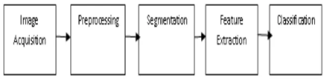
The CAD system consists of five stages such as acquisition of TRUS image of prostate, preprocessing, segmentation, feature extraction and classification. It is developed for automatic detection of prostate tumor in Transrectal Ultrasound (TRUS) image. The overview of the CAD system is depicted in figure 1. It can provide the valuable viewpoint and accuracy of earlier prostate cancer detection.

Figure 1: CAD System

follows: section 2 deals about image acquisition and preprocessing of original TRUS medical image of prostate. The DBSACN clustering with morphological operators for locating the Region of Interest (ROI) from TRUS prostate medical image is described in section 3. The feature extraction through Histogram, GLCM, and GLRLM are illustrated in section 4. The SVM classifier is discussed in section 5. The experimental analysis and discussion are presented in the section 6. Section 7 concludes this work with directions for further research.

2. Image Acquisitions and Preprocessing

Ultrasound imaging is a widely used technology for prostate cancer diagnosis and prognosis among the different medical image modalities. Image acquisition processes required less than 30 minutes for each case. The TRUS images of the prostate gland are acquired while the TRUS probe is supported and manipulated by the TRUS Robot using a joystick located next to the console, without the need for a dedicated assistant. The entire prostate is scanned by rotating the TRUS probe about its axis, minimizing prostate displacement and deformation. The probe depth can be manually adjusted by a surgeon. Accurate recording of images and corresponding TRUS frame coordinates were obtained. The gathered information is used in offline for the ultrasound image of the prostate gland. Image acquisition is done from ultrasound device via frame grabber. Image of the prostate can be generated using a series of TRUS images.

The ultrasound images are very difficult to process and analysis, because of poor image contrast, speckle noise and missing or diffuse boundaries in the Transrectal Ultrasound (TRUS) images. The data dropout noise is generally referred to as speckle noise [25, 26]. It is, in fact, caused by errors in data transmission. The corrupted pixels are either set to the maximum value, which is something like a snow in image or have single bits flipped over. This kind of noise affects the ultrasound images [8]. To interpret the TRUS images, preprocessing is necessary to improve the quality of image and make the subsequent phases as an easier and reliable one. The M3-Filter is used to generate a despeckled image that maintained proteomic while suppressing unwanted features in the image [7]. Once the noise is removed to enhance the contrast of the image, the imtophat filter is used to create with required edges. Since, the information of edges is needed for the proper segmentation. Then enhanced image is segmented using DBSCAN clustering with morphological operators discussed in the following section.

3. Extraction of Region of Interest (RoI)

The RoI is extracted using the DBSCAN clustering with morphological operators from thresholded image which is obtained by applying Local Adaptive Thresholding method in order to reduce the complexity of segmentation process. The schematic diagram of RoI extraction is shown in figure 2 and its detailed description is given subsequent sections.

Figure 2: Schematic diagram for ROI

3.1 Local Adaptive Threshold

The enhanced image is thresholded by using local adaptive method. The mean value of the sub image is used as the threshold value for the pixel and works well in strict cases of the images that have approximately half to the pixels belonging to the objects and the other half to background. Threshold image g(x, y) can be defined:

1 i f f ( x , y ) < T g ( x , y )

0 o t h e r w i s e

 

  

 

The binary image obtained after thresholding contains several blocks holes. The morphological operators such as opening and closing are applied with large structuring element to isolate the object that is corresponding to the prostate region.

3.2 Morphological operators

Morphological operations are important in the digital image processing, since that can rigorously quantify many aspects of the geometrical structure of the way that agrees with the human intuition and perception [9, 10]. It emphasizes on studying geometry structure of image. The relationship between each part of image can be identified when processing image with morphological theory. Accordingly, the structural character of image in the morphological approach is analyzed in terms of some predetermined geometric shape known as structuring element [9]. The morphological operators opening and closing are defined as follows:

A  B = ( A  B )  B

A  B = ( A  B )  B

area must be isolated from other white regions in the thresholded image is a difficult task in TRUS prostate medical images.

3.3 DBSCAN Clustering

With the aim of separating background from TRUS image to target possible prostate, pixels of thresholded images are grouped by using DBSCAN. It takes a binary image, and delineates only significantly important regions. The expected outcome is desired boundary of the TRUS prostate image. The DBSCAN Algorithm for segmentation is detailed in figure 3. Technically, this algorithm is appropriate to tailor density based algorithm in which cluster definition guarantees that the number of positive pixels is equal to or greater than minimum number of pixels (MinPxl) in certain neighborhood of core points. The core point is that the neighborhood of a given radius (Eps) may contain at least a minimum number of positive pixels (MinPxl), i.e., the density in the neighborhood should exceed pre-defined threshold (MinPxl) [11, 12].

DBSCAN Algorithm

INPUT: Enhanced TRUS prostate image

OUTPUT: Segmented image which contains only prostate Step1: Set epsilon (Eps) and minimum points (MinPts).

Step2: Starts with an arbitrary starting point that has not been visited and then finds all the neighbor points within distance Eps of the starting point.

Step3: If the number of neighbors is greater than or equal to MinPts, a cluster is formed. The starting point and its neighbors are added to this cluster and the starting point is marked as visited. The algorithm then repeats the evaluation process for all the neighbors recursively.

Step4: If the number of neighbors is less than MinPts, the point is marked as noise.

Figure 3: DBSCAN Algorithm

4. Feature Extraction

Texture is one of the most important characteristics of an image. It is used to describe the local spatial variations in image brightness which is related to image properties such as coarseness, and regularity. This is achieved by performing numerical manipulation of digitized images to get quantitative measurements. Texture analysis can potentially expand the visual skills of the expert eye by extracting image features that are relevant to diagnostic problem and not necessarily visually extractable. In order to capture the spatial dependence of gray-level values which contribute to the perception of texture, a two-dimensional dependence texture analysis matrix is discussed for texture consideration. Since texture shows

its characteristics by both each pixel and pixel values. Normally texture analysis can be grouped into four categories: model-based, statistical-based, structural-based, and transform-based methods. Model-based methods are based on the concept of predicting pixel values based on a mathematical model. Statistical methods describe the image using pure numerical analysis of pixel intensity values. Structural approaches seek to understand the hierarchal structure of the image. Transform approaches generally perform some kind of modification to the image, obtaining a new “response” image that is then analyzed as a representative proxy for the original image [16].

This paper only focuses on statistical approaches, which represent texture with features that depend on relationships between the grey levels of the image. It is very helpful to know that different tissues have different textures [13]. Benign tumors are described as regular masses with homogenous internal echoes, while carcinomas are masses with fuzzy borders and heterogenous internal echoes. Statistical features are used in this paper where different texture features are constructed from the identified regions of interest of the TRUS images. In statistical texture analysis, texture features are computed from the statistical distribution of observed combinations of intensities at specified positions relative to each other in the image. Depending on the number of pixels in each combination, statistics are classified into first-order, second-order and higher-order statistics. A typical TRUS image of prostate contains a vast amount of heterogeneous information that depicts different parts. In order to build a robust diagnostic system towards correctly classifying normal and abnormal, we have to present all the available information that exists in TRUS image to the diagnostic system so that it can easily discriminate between the normal and the abnormal tissue [14, 15]. In this paper, segmented image (ROI) is utilized to construct the feature sets using Histogram method, Gray-Level Run-Length Method (GLRLM), and Grey-Level Co-occurrence Matrix (GLCM). And then each features set and the various combinations of them used for the classification. In this paper we analyze TRUS images using three different texture extraction methods. Performance of the combinations of the above three methods are also analyzed.

4.1 Intensity Histogram Features

and hence, the characteristic of an image can be expressed using the following measurements [17].

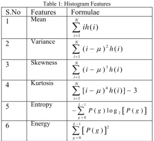
Mean reveals the general brightness of an image. Bright image should have high mean while dark image should have low mean, and also mean values characterize individual calcifications. Standard deviation or variance reveals the contrast of an image. Image with good contrast should have high variance. Standard Deviations (SD) also characterize the cluster. Skew measures is how asymmetry (unbalance) the distribution of the gray level. Image with bimodal histogram distribution (object in contrast background) should have high variance but low skew distribution (one peak at each side of mean). Energy measurement is closely related to skew. Highly skew distribution usually gives high-energy measurement. Entropy measures the average number of bits to code each gray level. It has inverse relationship with skew and energy measurement. Highly skew distribution tends to yield low Entropy. These are summarized in Table 1. Within ROI (ie segmented prostate region) a histogram distribution of the image is computed. Then six features are calculated for classification.

Table 1: Histogram Features S.No Features Formulae 1 Mean

1 ( )

N

i

ih i





2 Variance ₂ 1

( ) ( )

N

i

i  h i 





3 Skewness 3 1

( ) ( )

N

i

i  h i 





4 Kurtosis 4 1

[ ) ( )] 3

N

i

i  h i 

 



5 Entropy 1

_

_

0

( ) l o g ( )

L

g

P g P g









6 Energy 1

_

_

0

( )

L

g P g 





4.2. Gray Level Cooccurrence Matrix

The Gray Level Coocurrence Matrix (GLCM) method is a way of extracting second order statistical texture features [15, 18]. It models the relationships between pixels within the region by constructing Gray Level Co-occurrence Matrix. The GLCM is based on an estimation of the second-order joint conditional probability density functions p(i, j | d, θ) for various directions θ = 0, 45, 90, 135°, etc., and different distances, d = 1, 2, 3, 4, and 5. The function p(i, j | d, θ) is the probability that two pixels, which are located with an intersample distance d and a

direction θ, have a gray level i and j. The spatial relationship is defined in terms of distance d and angle θ. If the texture is coarse, and distance d is small, the pair of pixels at distance d should have similar gray values. Conversely, for a fine texture, the pairs of pixels at distance d should often be quite different, so that the values in the GLCM should be spread out relatively uniformly [19, 20]. Similarly, if the texture is coarser in one direction than another, then the degree of spread of the values about the main diagonal in the GLCM should vary with the direction θ [21]. The figure 3 represents the formation of the GLCM of the grey-level (4 levels) image at the distance d = 1 and the direction θ = 0°.

Figure 3(a): image with 4 grey level 3(b): GLCM for d = 1 and θ = 0°

The thin box in figure 3(a) represents pixel-intensity 0 with pixel intensity 1 as its neighbour in the direction θ = 0º. There are two occurrences of such pair of pixels. Therefore, the GLCM matrix formed with value 2 in row 0 and column 1. This process is repeated for other pair of intensity values. As a result, the pixel matrix represented in Figure 3(a) can be transformed into GLCM as shown in Figure 3(b). In addition to the direction (0º), GLCM can also be formed for the other directions 45º, 90º and 135º as shown in Figure 4.

Figure 4: Direction of GLCM generation.

The pixels 1, 2, 3 and 4 are representing the directions (θ) 0º, 45º, 90º and 135º respectively for distance d = 1 from the pixel x.

4.3. Gray-Level Run-Length Matrix

the texture features can be extracted for texture analysis [22]. It is a way of searching the image, always across a given direction, for runs of pixels having the same gray level value. Run length is the number of adjacent pixels that have the same grey intensity in a particular direction. Gray-level run-length matrix is a two-dimensional matrix where each element is the number of elements j with the intensity i, in the direction θ.

Thus, given a direction, the run-length matrix measures for each allowed gray level value how many times there are runs of, for example, 2 consecutive pixels with the same value. Next it does the same for 3 consecutive pixels, then for 4, 5 and so on. Note that many different run-length matrices may be computed for a single image, one for each chosen direction. The GLRLM is based on computing the number of gray level runs of various lengths [23]. A gray level run is a set of consecutive and collinear pixel points having the same gray level value. The length of the run is the number of pixel points in the run. The gray level run-length matrix is as follows.

R () = (g (i, j) |  ), 0 ≤ i ≤ Ng , 0 ≤ j ≤ Rmax ;

where Ng is the maximum gray level and Rmax is the maximum length. Figure 5 shows the sub image with 4 gray levels for constructing the GLRLM. Figure 6 shows that the GLRLM in the direction of 0 of the sub image in Figure 5.

1  2  3  4 

1  3  4  4  3  2  2  2 

4  1  4  1 

Figure 5: Matrix of Image

Gray  Level 

Run Length(j) 

1  2  3  4 

1  4  0  0  0 

2  1  0  1  0 

3  3  0  0  0 

4  3  1  0  0 

Figure 6: GLRL Matrix

In addition to the 0º direction, GLRLM can also be formed in the other direction, i.e. 45º, 90º or 135º.

Figure 7: Run Direction

Table 1: GLRLM Features

S.No Features Formulae

1 Short Run Emphasis (SRE) ₂

,

1 ( , )

i j

p i j

n



2 Long Run Emphasis (LRE) 2 ,

1

( , )

i j

j p i j n



3 Grey Level Non-uniformity

(GLN)

2

1

( , )

i j

p i j n

 

 

 

 

4 Run Length Non-uniformity 2

1

( , )

i i

p i j n

 

 

 

 

, ( , ) i j

n p i j j



2 ,

1 ( , )

i j p i j n



7 High Grey Level Run

Emphasis (HGRE) 2 ,

1

( , )

i j

i p i j n



Seven texture features can be extracted from the GLRLM. These features uses grey level of pixel in sequence and is intended to distinguish the texture that has the same value of SRE and LRE but have differences in the distribution of gray levels. Once features sets are constructed using Histogram features, GLCM, GRLM, and their combination. Then the next section explicates SVM classifier for the classification of extracted features.

5. Classification

set of cardinality n (n=|F|). For classification, the SVM is adapted and its detailed description is given below.

5.1 SVM Classifier

Support vector machine is based on statistical learning technique which is well-founded in modern statistical learning theory [27]. The Support Vector Machines were introduced by Vladimir Vapnik and his colleagues. The earliest mention was in (Vapnik, 1979). SVM is a useful technique for data classification [28]. It is also be a leading method for solving non-linear problem. A classification task usually involves with training and testing data which consist of some data instances. Each instance in the training set contains one target values and several attributes. The goal of SVM is to produce a model which predicts target value of data instances in the testing set which are given only the attributes. Classification in SVM is an example of Supervised Learning. Known labels help indicate whether the system is performing in a right way or not. This information points to a desired response, validating the accuracy of the system, or be used to help the system learn to act correctly. A step in SVM classification involves identification as which are intimately connected to the known classes [24].

Support vector machines use the training data to crate the optimal separating hyperplane between the classes. The optimal hyperplane maximizes the margin of the closest data points. A good separation is achieved by the hyperplane that has the largest distance to the nearest training features of any class (so-called functional margin). Maximum-margin hyperplane and margins for a SVM trained with samples from two classes. Samples on the margin are called the support vectors (Fatima Eddaoudi, and Fakhita Regragui,: 2011). SVM divides the given data into decision surface. Decision surface divides the data into two classes like a hyper plane. Training points are the supporting vector which defines the hyper plane. The basic theme of SVM is to maximize the margins between two classes of the hyper plane (Steve, 1998).

Basically, SVMs can only solve binary classification problems. They have then been extended to handle multi-class problems. The idea is to decompose the problem into many binary-class problems and then combine them to obtain the prediction. To allow for multi-class classification, SVM uses the one-against-one technique by fitting all binary sub classifiers and finding the correct class by a voting mechanism.

The “one-against-one" approach (Knerr et al., 1990) is implemented in SVM for multiclass classification. If K is the number of classes, then K(K - 1)/2 binary classifiers

are constructed and trained to separate each pair of classes against each other, and uses a majority voting scheme (max-win strategy) to determine the output prediction. For training datafrom the i th and the j th classes, we solve the following two-class classification problem ( Metehan Makinacı: 2005). Let us denote the function associated with the SVM model of

{

c c

}

( )

( ( ) )

g x



sign f x

An unseen example, x, is then classified as:

1 1

( )

arg max

( )

K K

ij i

i j i j

f x

V x

   



 

where:

,

( )

1

1

( )

( )

1

0

ij i j

ij

g x

if

V

x

g x

if





 

_{ }



Each feature set is examined using the Support Vector Machine classifier. In classification, we use a voting strategy: each binary classification is considered to be a voting where votes can be cast for all data points x in the end point is designated to be in a class with the maximum number of votes. In case that two classes have identical votes, though it may not be a good strategy, now we simply choose the class appearing first in the array of storing class names.

The objective of any machine capable of learning is to achieve good generalization performance, given a finite amount of training data, by striking a balance between the goodness of fit attained on a given training dataset and the ability of the machine to achieve error-free recognition on other datasets. With this concept as the basis, support vector machines have proved to achieve good generalization performance with no prior knowledge of the data. The optimal separating hyperplane can be determined without any computations in the higher dimensional feature space by using kernel functions in the input space. Commonly used kernels include:

Linear Kernel:

K x y

( , )



x y

.

Radial Basis Function (Gaussian) Kernel:

2 2

( - ||x - y || / 2 )

K ( x , y ) = e 

Polynomial Kernel:

d

K(x, y) = (x.y + 1)

6. EXPREMENT ANALYSIS AND

DISCUSSION

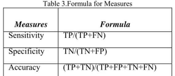
Algorithms discussed in the previous sections have been implemented using MATLAB. The intact of 5500 images in normal and abnormal categories which are transformed into histogram, Gray Level Cooccurrence matrix (GLCM) and Grey Level Run-Length matrix (GLRLM). The nine histogram features, twenty two GLCM features and eleven GRLM features are extracted from the corresponding models respectively. The performance of various texture models are analyzed by using statistical parameters such as sensitivity, specificity, accuracy and discussed. The statistical parameters with formula are given in Table 3.

Table 3.Formula for Measures

Measures Formula

Sensitivity TP/(TP+FN) Specificity TN/(TN+FP) Accuracy (TP+TN)/(TP+FP+TN+FN)

TP- predicts cancer as cancer. FP - predicts cancer as normal. TN - predicts normal as normal. FN - predicts normal as cancer

Sensitivity and Specificity are the two most important characteristics of a medical test. Sensitivity is the probability that the test procedure declares an affected individual affected (probability of a true positive). Specificity is the probability that the test procedure declares an unaffected individual unaffected (probability of a true negative). Accuracy measures the quality of the classification. It takes into account true and false positives and negatives. Accuracy is generally regarded with balanced measure whereas sensitivity deals with only positive cases and specificity deals with only negative cases. TP is number of true positives, FP is number of false positives, TN is number of true negatives and FN is number of false negatives. A confusion matrix provides information about actual and predicted cases produced by classification system. The performance of the system is examined by demonstrating correct and incorrect patterns. They are defined as confusion matrix in Table 4.

Table 4.Confusion Matrix

The higher value of both sensitivity and specificity shows better performance of the system. The constructed feature sets are separately tested using the SVM classifier. The computational results are presented in Table5.

Table 5: computational results

Methods sensitivity Specificit

y Accuracy

Histogram 0.81090909 0.9979591 0.82978333 GLRLM 0.82495575 1.0000000 0.85000000 GLCM 0.83790900 1.0000000 0.87895500 GLRLM+HIST 0.84615384 0.9992960 0.89683333 GLCM+HIST 0.84745762 1.0000000 0.90700000

GLCM+GLRLM 0.86206896 1.0000000 0.91333333 ALL 0.91743119 1.0000000 0.92833333

The results in Table 5 shows that the texture features extracted from different models discriminate malignant and benign with different accuracy. The individual performance measures are exposed in figure 5(a) – 5(c).

Figure 5(a): performance of sensitivity

Figure 5(b): performance of specificity

Figure 5(c): performance of accuracy Actual Predicted

Positive Negative

Positive TP FP

From the table 5, we observed that the maximum and minimum classification accuracies are 93% and 83% with SVM classifier. The histogram features discriminate between malignant masses and benign masses on TRUS prostate images with 83% accuracy, 81% sensitivity and 99% specificity levels that are relatively poorer compare to others. GLRLM features yielded an accuracy of 85% for distinguishing malignant and benign masses on TRUS prostate images. It is 2% higher than features based on histogram. The GLCM features achieved an accuracy of 88% where 84% sensitivity and 100% specificity. The accuracy of GLCM features 3% higher than GLRLM feature and 5% higher than Histogram features.

The combination of Histogram features and GLRLM features is achieved 90% of the accuracy, where as 91% of accuracy is produced when combined the Histogram features with GLRLM features. The accuracy difference between these two methods is only 1% even while the sensitivity and specificity of these two are almost same 85% and 100% respectively.The accuracy of 91 % is arrived by the combination of GLCM features and GLRLM features, whilst 86% sensitivity and 100% specificity. The predicted accuracy is 5%, which is 3% higher than GLRLM, GLCM respectively. The combination of Histogram features, GLCM features and GLRLM features produces the highest accuracy of 93%, 91% sensitivity, and 100% specificity followed by GLCM features combined with GLRLM features with the accuracy of 91%, 86% sensitivity, and 100% specificity.

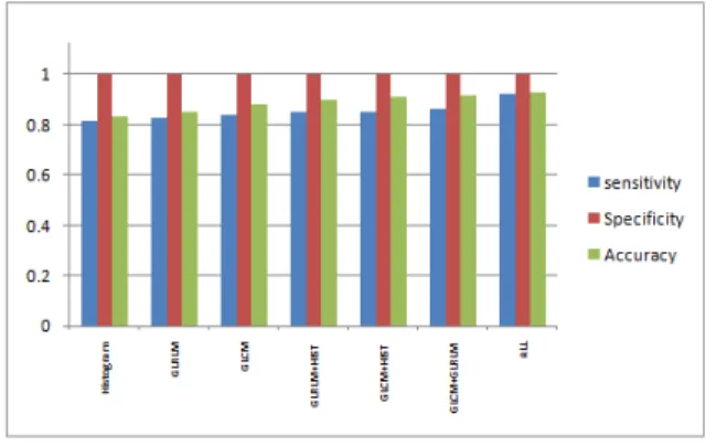
Figure 6: Relative performance measures

The Figure 6 shows that the relative performance measures with respect to proposed methods. By considering the different texture methods independently, it is not able to confirm that there is a universal method for best classification. However, usually the statistical cooccurrence (GLCM) features are used. The combination of various methods features produces a significant increase in the accuracy levels. It is interesting to note that using combined features

produces relatively good classification results. The percentage of accuracy of combined features is higher than the values obtained from others. These analyses conclude that the combination of Histogram, GLCM and GLRLM texture features achieves best classification accuracy for distinguishing between malignant masses and benign masses on TRUS prostate images.

7. Conclusion

Texture analysis is a potentially valuable and versatile in TRUS imaging for prostate cancer interpretation. In some cases, radiologists face difficulties in directing the tumors. In this work, feature extraction methods for the TRUS prostate cancer classification problem and an innovative approach (combined features) of finding the malignant and benign masses from the TRUS prostate medical images are proposed and analyzed. The performances of classifiers for the texture-analysis methods are evaluated using various statistical parameters such as sensitivity, specificity and accuracy. The experiment results show that there is considerable performance variability among the various texture methods. The histogram features and GLRLM features performances are considerably poor. The combination histogram features, GLRLM features and GLCM features outperformed well in discriminating between or among prostate cancer. Using proper feature selection method accuracy may be improved efficiently in future.

References

[1] Vidhi Rawat ,Alok jain, and Vibhakar shrimali: “Investigation and Assessment of Disorder of Ultrasound B-mode Images” (IJCSIS) International Journal of Computer Science and Information Security, Vol. 7, No. 2, February 2010, PP.289 – 293.

[2] Ransohoff DF, McNaughton Collins M, Fowler FJ. Why is prostate cancer screening so common when the evidence is so uncertain? A system without negative feedback. Am J Med. 2002 Dec 1;113(8):663-7. Review

[3] Grossfeld GD, Carroll PR. Prostate cancer early detection: a clinical perspective. Epidemiol Rev. 2001;23(1):173-80. Review.

[4] Cookson MM. Prostate cancer: screening and early detection. Cancer Control. 2001 Mar-Apr;8(2):133-40. Review

[5] Ferdinand Frauscher: “Contrast-enhanced Ultrasound in Prostate Cancer” Imaging and Radiotherapy, © T O U C H B R I E F I N G S 2 0 0 7. Pp 107-108.

[6] Ethan J Halpern, MD: “Contrast-Enhanced Ultrasound Imaging of Prostate Cancer”,

[8] Sinha, G.R., Kavita Thakur and Kowar, M.K. (2008). “Speckle reduction in Ultrasound Image processing”, Journal of Acoustical. Society of India, Vol. 35, No. 1, pp. 36-39. [9] Anil K. Jain. (1989) Fundamentals of Digital Image

Processing: Prentice Hall.

[10] Gonzalez, R. and Woods, R. (2002). Digital Image Processing. 3rd Edn., Prentice Hall Publications, pp. 50-51. [11] Ester, M., Kriegel, H.P., Sander, J., and Xu, X.(1996) ‘A

density-based algorithm for discovering clusters in large spatial databases with noise’. Proceedings of 2nd International Conference on Knowledge Discovery and Data Mining, Portland: AAAI Press. pp. 226-231.

[12] Sinan Kockara, Mutlu Mete, Bernard Chen, and Kemal Aydin:(2010). ‘Analysis of density based and fuzzy c-means clustering methods on lesion border extraction in dermoscopy images’, From Seventh Annual MCBIOS Conference: Bioinformatics Systems, Biology, Informatics and Computation Jonesboro, AR, USA. pp. 19 - 20.

[13] Amadasun, M. and King, R., (1989) ‘Textural features corresponding to textural properties’, IEEE Transactions on Systems, Man, and Cybernetics, vol. 19, no. 5, pp. 1264 - 1274.

[14] Haralick, R.M. , Shanmugan, K.. and Dinstein, I.( 1973) ‘Textural Features for Image Classification’, IEEE Tr. on Systems, Man, and Cybernetics, Vol SMC-3, No. 6, pp. 610-621.

[15] Haralick, R.M. (1979) ‘Statistical and Structural Approaches to Texture’, Proceedings of the IEEE, Vol. 67, No. 5, pp. 786-804.

[16] Mohamed, S.S. and Salama M.M. ( 2005 ) ‘Computer Aided diagnosis for Prostate cancer using Support Vector Machine’ Publication: Proc., medical imaging conference, California, SPIE Vol. 5744, pp. 899-907.

[17] Chitrakala, S. Shamini, P. and Manjula, D: “Multi-class Enhanced Image Mining of Heterogeneous Textual Images Using Multiple Image Features” , Advance Computing Conference, 2009. IACC 2009. IEEE International , 2009 , Page(s): 496 – 501.

[18] Haralick R. M., Shanmugam K., Dinstein I. Textural Features of Image Classification. IEEE Transactions on Systems, Man and Cybernetics. 1973. Vol. 3(6). P. 610-621. [19] Soh L., Tsatsoulis C. Texture Analysis of SAR Sea Ice

Imagery Using Gray Level Co-Occurrence Matrices. IEEE Transactions on Geoscience and Remote Sensing. 1999. Vol. 37(2). P. 780 – 795.

[20] Clausi D A. An analysis of co-occurrence texture statistics as a function of grey level quantization. Canadian Journal of Remote Sensing. 2002. Vol. 28(1). P. 45-62.

[21] A. Sakalauskas, A. Lukosevicius1, and K. Lauckaite: “Texture analysis of transcranial sonographic images for Parkinson disease Diagnostics” ISSN 1392-2114 ULTRAGARSAS (ULTRASOUND), Vol. 66, No. 3, 2011. Pp 32 – 36.

[22] K.Thangavel, M.Karnan, R.Sivakumar and A. Kaja Mohideen “ Ant Colony System for Segmentation and Classification of Microcalcification in Mammograms” AIML Journal, Volume (5), Issue (3), pp.29-40., September, 2005. [23] Jong Kook Kim, Jeong Mi Park, Koun Sik Song and Hyun

Wook Park “Texture Analysis and Artificial Neural Network for Detection of Clustered Microcalcifications on Mammograms” IEEE, pp.199 – 206, 1997.

[24] Devendran V et. al., “Texture based Scene Categorization using Artificial Neural Networks and Support Vector Machines: A Comparative Study,” ICGST-GVIP, Vol. 8, Issue IV, pp. 45-52, December 2008.

[25] L. Gagnon and F.D. Smaili: 'Speckle Noise Reduction of Airborne SAR Images with Symmetric Daubechies Wavelets', SPIE Proc. #2759, pp. 1424,1996.

[26] H. Guo, J E Odegard, M.Lang, R.A.Gopinath, I.W.Selesnick, and C.S. Burrus, “Wavelet based Speckle reduction with application to SAR based ATD/R”, First Int’I Conf. on image processing , vol. 1, pp. 75-79,Nov 1994. [27] Vapnik V. (1995). The Nature of Statistical Learning

Theory, chapter 5. Springer-Verlag, New York.

[28] Vapnik.V, Statistical Learning Theory. John Wiley & Sons, New York, 1998.

Manavalan Radhakrishnan obtained M.Sc., Computer Science from St. Joseph’s College of Bharathidasan University,Trichy, Tamilnadu, India, in the year 1999, and M.Phil., in Computer Science from Manonmaniam Sundaranar University, Thirunelveli, Tamilnadu, India in the year 2002. He works as Asst.Prof & Head, Department of Computer Science and Applications, KSR College of Arts and Science, Thiruchengode, Nammakal, Tamilnadu, India. He pursues Ph.D in Medical Image Processing. His areas of interest are Medical image processing and analysis, soft computing, pattern recognition and Theory of Computation.