Random Walk Models Classifications: An Empirical Study for Malaysian Stock Indices

ISSN 1546-9239

© 2008 Science Publications

Corresponding Author: Chin Wen Cheong, Faculty of Information Technology, Multimedia University, 63100 Cyberjaya,

Random Walk Models Classifications: An Empirical Study for Malaysian Stock Indices

Chin Wen Cheong

Faculty of Information Technology

Multimedia University, 63100 Cyberjaya, Selangor, Malaysia

Abstract: This article studied the Random Walk models introduced by Campbell et al.[2] for Malaysian stock market. The analysis is implemented under the possible drastic economics structural change using an iterative structural change test. After the break-date identification, the random walk hypothesis is tested by multiple variance ratios test in two separate periods. We further examined the serial correlations of return’s squared innovations for random walk classifications. Our empirical results evidenced the random walk type 3 dominating most of the Malaysian stock indices.

Keywords: structural break, market efficiency, stock market, unit root test, random walk.

INTRODUCTION

Informationally efficiency is often used to describe how all relevant information is impounded into the security prices of financial markets. Fama’s[1] weak-form efficient market hypothesis (EMH), which is our focus, stated that the current asset price is determine only by its historical prices (information set) of that particular asset. If stock price failed to reject the random walk hypothesis (RWH), this implies that the future returns are unpredictable by using information on past returns. On the other hand, if the stock prices is characterised by a mean reverting (trend stationary) process, then there is a tendency for the price level to return to its trend path. This suggests that the presence of predictable component based on the historical information. Campbell et al.[2] further this study by distinguishing the random walk processes into three sub-hypotheses. The random walk 1(RW1) is the most restrictive model which requires independent and identically distributed (i.i.d) of the price changes. In random walk 2(RW2), the restriction of identically distributed condition is not imposed. Therefore, the unconditional heteroscedasticity is allows in the increments. Finally, by relaxing the independence restriction of RW2, the RW3 model is obtained. RW3 is actually further examines the possible of serial correlation in the squared increments which leads to the presence of conditional heteroscedasticity. This conditional volatility is well modeled by ARCH models introduced by Engle[3] and Bollerslev[4] among others. It is worth noted that RW3 contains RW1 and RW2 under special conditions. The implication of RWH sometimes

can provide insight understanding of efficiency market hypothesis (EMH). However, the RWH can only be treated as equivalent to EMH under the risk neutrality condition. Investors, economists and econometricians have shown considerable interests to identify these processes which are important in their investments, implication of market efficiency and developing correct model specifications.

As an emerging stock market, Kuala Lumpur stock exchange (KLSE) has received great attentions from researchers and investors[5-8] as the case studies and potential investment alternatives. For structural break analysis, Chaudhuri and Wu[9] reject the null hypothesis of random walk in KLSE using 12 years monthly stock prices among the other 17 emerging markets. Goh et al. [10]

This study evaluates the possible type of random walk in the Kuala Lumpur Stock Exchange (KLSE) and the nine sectoral indices before and after the periods of Asia financial crisis. The ten selected stock indices consist of KLCI and nine major multi-sectors such as industrial(IND), industrial product(INP), consumer products(COP), construction(CON), mining(MIN), finance(FIN), properties(PRO), plantation(PLA) and trading/services(TRA) respectively. The Technology and Syariah indices are not included in our empirical analysis due to the unavailability (begin at year 2000) and overlapping listed companies which initially exist in other sectors respectively. We firstly examine the random walk hypothesis using the multiple variance ratios. Each of the indices is group accordingly follows the Campbell et al.[2] random walk processes namely the homoscedasticity RW (RW1), heteroscedasticity RW (RW2) respectively. For RW 3, even though the returns series commonly follow the random walk hypothesis with uncorrelated innovations, but their squared innovations often exhibit the presence of serial correlations. This phenomena is also named as the conditional heteroscedasticity effect which introduced by Engle[3]. After the classifications of RW, we can utilize the predictable component based on the historical information that may assist investors to produce above average profits.

Daily closing transaction price indices have been selected from 1996 to 2006 which covers before and after the Asian crisis. All the data are collected from the DATASTREAM with 2578 observations for each series. During this period, the KLSE composite index (CI) come under severe pressure and encountered drastic fall in price level. One of the objectives of this study is to examine whether the nine sectoral indices follow the behaviour of the KLCI. The specific day of the structural break is determined by an iterative Chow’s test introduced by Andrews[13] tests. Alternatives for unknown break location test are such as CUSUM test by Brown et al [14] and Bai and Perron[15] using UDMax and WDMax statistics among others.

METHODOLOGY

Multiple Variance Ratios test: Lo and MacKinlay[16] focus on individual variance ratio test for a specific interval in random walk hypothesis. LOMAC conclude that in a finite sample the increments in the variance are linear in the observation interval for a random walk. Lets a sample size of nq+1 observations(p0, p1, …., pnq)

at equally spaced intervals, where q is any integer greater than 1 and nq is the number of observations of

pt. The variance of a qth-differenced variable is q time

as large as the first differenced variable. The idea can be illustrated in the form of:

V(pt- pt-q) = qV(pt- pt-1), (1)

where q is any positive integer. The variance ratio can further written as:

) 1 ( ) ( ) ( ) ( ) ( ₂ 2 1 1 σ σ q p p V p p V q VR t t q t t q = − − = − −

. (2)

The unbiased estimators σ2(1) and σ2(q) are denoted as:

) 1 ( ) ˆ ( ) 1 ( ˆ 1 2 1 2 − − − = = − nq p p nq k k k µ

σ ; (3)

m q p p q nq q k q k k = − − − = 2 2 ) ˆ ( ) ( ˆ µ

σ ; (4)

where ˆ 1 (p p₀)

nq nq−

=

µ and ( 1 )(1 )

nq q q nq q

m= + − − .

Two alternative test statistics Z(q) and Z*(q) with the assumption of homomskeastic and heteroskedastic increments random walk respectively. If the null hypothesis of homoskedastic increments of random walk is not rejected, the associated test statistics has an asymptotic standard normal distribution as follows:

) ( ˆ 1 ) ( ) ( 0 q q VR q Z σ −

= , (5)

where 2 1 ) ( 3 ) 1 )( 1 2 ( 2 ) (

ˆ₀ = − −

nq q

q q q

σ . On the other hand,

the associate test statistic for heteroskedastic increments random walk, Z*(q) is given as follows:

) ( ˆ 1 ) ( ) ( * _* q q VR q Z e σ −

= ; (6)

where 2 1 ˆ 1 4 ) ( ˆ 2 1 1 * − = − = k q k e q k q φ

σ (7)

− − − − − − = = − + = − − − − nq j j j nq k j k j k j j j k p p p p p p 1 2 1 1 2 1 2 1 ) ˆ ( ) ˆ ( ) ˆ ( ˆ µ µ µ

φ . (8)

comparison of the varied set of variance ratio estimates with unity. Consider a set of variance ratio estimates,

} ,..., 2 , 1 | ) (

ˆ _{q i m}

M_{r i} = , the random walk null hypothesis test a set of sub-hypothesis, H0i : Mr(qi) = 0 and H1i : Mr(qi) ≠ 0. Since any rejection of H0i will lead to the rejection of the random walk null hypothesis, only the maximum absolute value in the set of test statistics is highlighted. The largest absolute value of the test statistics are defined using the following probability inequality:

P

[

]

where the SMM(α;m;N) is the upper α point of Studentized Maximum Modulus(SMM) distribution with parameter m and N(sample size) degrees of freedom. Asymptotically, when sample size is extremely large(∞), the limiting SMM is:

2 / * ) ; ; (

lim SMM α m Zα

N→∞ ∞ = . (10)

The Zα_*/2 is the standard normal distribution with α*= 1-(1-α)1/m. Under the MVR test, the rejection of homoskedasatic random walk hypothesis (RW1) is based on whether the maximum absolute value of Z(q) is greater than the Studentized Maximum Modulus(SMM) critical value. This rejection concludes that the presence of either heteroskedastic or/and serial correlation in the equity price series. In the following test of heteroskedastic random walk (RW2), the rejection of heteroskedastic random walk leads us to the existence of autocorrelation in equity price series.

The presence of RW3 can be further justified using LM correlation test and Engle ARCH test respectively. The RW3 is tally with the conditional volatility which often occurs in financial asset pricing. The risk can be identified by including the conditional volatility in the mean equation as suggested by Engle et al. [18] ARCH-mean model.

RESULTS AND DISCUSSIONS

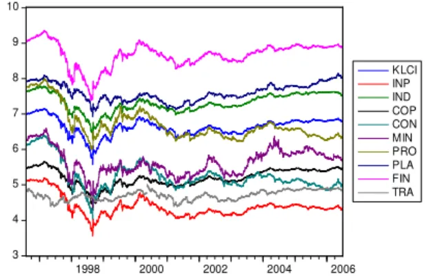
Fig. 1 illustrates the plots of natural log price index for all the studied indices and indicate that a similar structural change happened in all the indices within the year of 1997 to 1998. Other than that, the movements of the prices indices seem to be stable in general. In order to determine the exact location of the break date due to the Asian financial crisis, we run the

Andrews[13] test. Except the trading & service index, significant break points are found for all the other indices. The earliest break is experienced by the Property index (12/25/1997) during the crisis, follows by Finance (8/18/1998) and simultaneously by other indices at 9/2/1998, a day after the Malaysian government imposed the currency policy. Most of the indices rebounded significantly after the currency controls, for example, the KLCI radically increase by 12%, Construction 13%, Finance, Plantation, Industrial product, 9% and the lowest is 3% by Property.

3 4 5 6 7 8 9 10

1998 2000 2002 2004 2006

KLCI INP IND COP CON MIN PRO PLA FIN TRA

Fig. 1: Malaysian prices indices

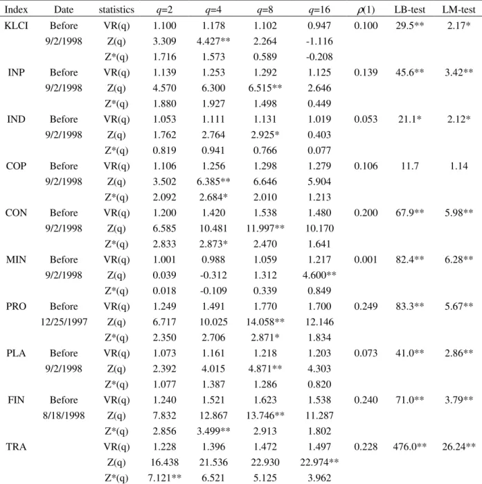
Multiple Variance Ratio Test

Table 1: Multiple Variance-Ratio Test before structural break

Index Date statistics q=2 q=4 q=8 q=16 ρ(1) LB-test LM-test KLCI Before VR(q) 1.100 1.178 1.102 0.947 0.100 29.5** 2.17*

9/2/1998 Z(q) 3.309 4.427** 2.264 -1.116 Z*(q) 1.716 1.573 0.589 -0.208

INP Before VR(q) 1.139 1.253 1.292 1.125 0.139 45.6** 3.42** 9/2/1998 Z(q) 4.570 6.300 6.515** 2.646

Z*(q) 1.880 1.927 1.498 0.449

IND Before VR(q) 1.053 1.111 1.131 1.019 0.053 21.1* 2.12* 9/2/1998 Z(q) 1.762 2.764 2.925* 0.403

Z*(q) 0.819 0.941 0.766 0.077

COP Before VR(q) 1.106 1.256 1.298 1.279 0.106 11.7 1.14 9/2/1998 Z(q) 3.502 6.385** 6.646 5.904

Z*(q) 2.092 2.684* 2.010 1.213

CON Before VR(q) 1.200 1.420 1.538 1.480 0.200 67.9** 5.98** 9/2/1998 Z(q) 6.585 10.481 11.997** 10.170

Z*(q) 2.833 2.873* 2.470 1.641

MIN Before VR(q) 1.001 0.988 1.059 1.217 0.001 82.4** 6.28** 9/2/1998 Z(q) 0.039 -0.312 1.312 4.600**

Z*(q) 0.018 -0.109 0.339 0.849

PRO Before VR(q) 1.249 1.491 1.770 1.700 0.249 83.3** 5.67** 12/25/1997 Z(q) 6.717 10.025 14.058** 12.146

Z*(q) 2.350 2.706 2.871* 1.834

PLA Before VR(q) 1.073 1.161 1.218 1.203 0.073 41.0** 2.86** 9/2/1998 Z(q) 2.392 4.015 4.871** 4.303

Z*(q) 1.077 1.387 1.286 0.820

FIN Before VR(q) 1.240 1.521 1.623 1.538 0.240 71.0** 3.79** 8/18/1998 Z(q) 7.832 12.867 13.746** 11.287

Z*(q) 2.856 3.499** 2.913 1.802

TRA VR(q) 1.228 1.396 1.472 1.497 0.228 476.0** 26.24**

Z(q) 16.438 21.536 22.930 22.974** Z*(q) 7.121** 6.521 5.125 3.962

Notes:

1. .Multiple variance ratios:

Z(q) denotes the homoskedasticity test statistics and Z*(q) denotes the hetoroskedasticity test statistics;

Only the maximum absolute value statistics are comparing with the Studentized Maximum Modules(SMM) critical value of 2.49 and 3.00 at the 5% and 1% level respectively;

2. According to LOMAC(1988) the first order autocorrelation coefficient is estimated by Mˆr(2)=VR(2)−1=ρˆ(1); * and ** indicate the maximum absolute Z(q) or Z*(q) with p<0.05 and p<0.01.

3. Random walk 3 evaluation:

Ljung Box Serial Correlation Test( Q-statistics):Null hypothesis – No serial correlation; LM ARCH test: Null hypothesis - No ARCH effect;

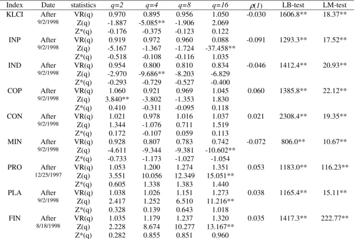
Table 2: Multiple Variance-Ratio Test after structural break

Index Date statistics q=2 q=4 q=8 q=16 ρ(1) LB-test LM-test KLCI After VR(q) 0.970 0.895 0.956 1.050 -0.030 1606.8** 18.37**

9/2/1998 _{Z(q) -1.887 -5.085** -1.906 2.069}

Z*(q) -0.176 -0.375 -0.123 0.122

INP After VR(q) 0.919 0.972 0.960 0.088 -0.091 1293.3** 17.52**

9/2/1998 _{Z(q) -5.167 -1.367 -1.724 -37.458**}

Z*(q) -0.518 -0.108 -0.116 1.035

IND After VR(q) 0.954 0.800 0.810 0.834 -0.046 1412.4** 20.93**

9/2/1998 _{Z(q) -2.970 -9.686** -8.203 -6.829}

Z*(q) -0.293 -0.729 -0.527 -0.400

COP After VR(q) 1.060 0.921 0.969 1.045 0.060 1385.8** 22.12**

9/2/1998 _{Z(q) 3.840** -3.802 -1.353 1.830}

Z*(q) 0.410 -0.311 -0.095 0.118

CON After VR(q) 1.021 0.978 1.016 1.037 0.021 2308.4** 19.35**

9/2/1998 _{Z(q) 1.344 -1.076 0.711 1.519}

Z*(q) 0.172 -0.107 0.059 0.113

MIN After VR(q) 0.928 0.807 0.783 0.742 -0.072 806.0** 10.67**

9/2/1998 _{Z(q) -4.611 -9.344 -9.381 -10.602**}

Z*(q) -0.733 -1.173 -1.027 -1.054

PRO After VR(q) 1.053 1.200 1.274 1.351 0.053 1183.0** 116.23**

12/25/1997 _{Z(q) 3.551 10.056 12.349 15.051**}

Z*(q) 0.605 1.338 1.383 1.440

PLA After VR(q) 1.038 1.026 1.151 1.273 0.038 1165.4** 15.11**

9/2/1998 _{Z(q) 2.417 1.252 6.510 11.216**}

Z*(q) 0.328 0.139 0.643 1.018

FIN After VR(q) 1.035 1.179 1.237 1.320 0.035 1417.3** 222.77**

8/18/1998 _{Z(q) 2.228 8.674 10.277 13.167**}

Z*(q) 0.282 0.855 0.851 0.960

Notes:

1. .Multiple variance ratios:

Z(q) denotes the homoskedasticity test statistics and Z*(q) denotes the hetoroskedasticity test statistics;

Only the maximum absolute value statistics are comparing with the Studentized Maximum Modules(SMM) critical value of 2.49 and 3.00 at the 5% and 1% level respectively;

2. According to LOMAC(1988) the first order autocorrelation coefficient is estimated by Mˆr(2)=VR(2)−1=ρˆ(1); * and ** indicate the maximum absolute Z(q) or Z*(q) with p<0.05 and p<0.01.

3. Random walk 3 evaluation:

Ljung Box Serial Correlation Test( Q-statistics):Null hypothesis – No serial correlation; LM ARCH test: Null hypothesis - No ARCH effect;

* and ** indicate p<0.05 and p<0.01.

order autocorrelations indicate relatively higher values as compare to others indices with the values of 0.249 (property), 0.240 (finance), 0.228 (trading&service), 0.200 (construction) and 0.106 (consumer product) respectively. However, the daily returns especially in emerging market may cause by the infrequent trading behaviour (Miller et al., [21]). According to Miller et al., this spurious autocorrelation can be adjusted using a first order autoregressive or moving average. Finally, the squared innovations serial correlations are examine using Ljung-Box serial correlation test and Engle ARCH test respectively. Except the Consumer product

index, all the indices show the evidence of dependence property in the squared innovation or conditional volatility.

categorized the remaining nine indices as RW3 which further verify the not identically distributed innovations (RW2) are correlated.

After the structural break: After the economic crisis and currency control, some significant changes are observed where the VR(q) for KLCI, Industrial product, Industrial and Mining indices are less than unity. The negatively serial correlation indicates that these indices are converted to mean-reverting processes as compare to mean-aversion before the structural change. Table 2 shows similar results before the structural break where only the Construction index failed to reject the homoscedastic random walk. After the structural change, all the indices failed to reject the heteroscedastic random walk. We conclude that only the Construction follows an independent and identical distributed random walk (RW1). Whereas, the remaining indices evidence the heteroscedastic random walks (RW2). Next, all the indices strongly reject the null hypothesis of no serial correlation in squared innovations and suggest the presence of RW3.

CONCLUSION

This paper studies the classification of random walk processes in the Malaysian stock markets. Our results demonstrate that Asian Crisis and currency control show instantaneous impacts to the Malaysian stock market in general. Some significant changes happened in KLCI, Industrial product, Industrial and Mining indices where the mean-aversion processes observed before the structural changes have transformed to mean-reverted processes. These findings imply that there are tendency for the price levels to return to its trend paths. This suggests that after the structural change, the mentioned indices consist of predictable component based on their historical information.

Our results (before and after break) also indicate that the RW2 unconditional heteroscedasticity increments are found to be correlated (squared increments) and lead us to conclude the presence of RW3. The RW3 suggests that even the squared increments of the returns series are predictable but the return increment still following an unpredictable random walk process. The dependence property of squared increments is widely used in financial time series analysis such as risk management, portfolio analysis and derivative pricing. The most prominent

application is the measurement of value-at-risk(VaR) in risk and portfolio analysis. As a result, we conclude that most of the Malaysian stock indices are in favour of RW3. For future work, we would like to look into the estimation and prediction of VaR for the Malaysian stock indices.

ACKNOWLEDGEMENT

Author would like to gratefully acknowledge financial support from the Multimedia University and the Research Design and Development and Innovation Grant (IP20070322007).

REFERENCES

1. Fama, E.F., 1965. The Behaviour of Stock Market Prices, Journal of Business, 38: 34-105.

2. Campbell, J.Y., Lo, A.W. and MacKinlay, A.C., 1997, The Econometrics of Financial Markets, Princeton, Princeton University Press.

3. Engle, R.F., 1982, Autoregressive conditional heteroskedasticity with estimates of the variance of United Kingdom inflation, Econometrica, 50(4), 987-1007.

4. Bollerslev, T., 1986. Generalized autoregressive conditional heteroskedasticity, Journal of Econometrics, 31, 307-327.

5. Annuar, M.N., M. Ariff and M. Shamsher, 1991. Technical analysis, unit root and weak-form efficiency of the K LSE, Banker’s Journal Malaysia, 64: 55-58.

6. Kok, K.L. and F.F. Lee, 1994. Malaysian second board stock market and the efficient market hypothesis, Malaysian Journal of Economic Studies, 31(2): 1-13.

7. Lim, K.P., M.S. Habibullah and H.A. Lee, 2003. A BDS test of random walk in the Malaysian stock market. Labuan Bulletin of International Business and Finance, 1(1): 29-39.

8. Chin W.C. and I. Zaidi, 2007. The impact of multiple structural-breaks on Malaysian Stock Market , E. J of. Econ. Fin. and Ad. Sc., 7: 94-103. 9. Chaudhuri, K., and Wu, Y., 2003. Random walk

10. Goh K.L., Y.C. Wong and Kok K.L., 2005. Financial crisis and intertemporal linkages across the ASEAN-5 stock markets, Review of Quantitative Finance and Accounting, 24: 359-377. 11. Vogelsang T.J., 1997. Wald type tests for detecting breaks in the trend function of a dynamic time series, Econometric Theory, 13: 818-849.

12. Lean H. H. and S. Russel, 2005. Do Asian stock markets follow a random walk? Evidence from LM unit root tests with one and two structural breaks, ABERU Discussion Paper 11, Monash University. 13. Andrews, D.W.K., 1993. Tests for parameter

instability and structural change with unknown change point, Econometrica, 61: 821-856.

14. Brown, R.L., J. Durbin, and J.M. Evans, 1975. Techniques for testing the constancy of regression relationships over time, Journal of the Royal Statistical Society Series B, 37: 149-192.

15. Bai, J and Perron, P., 1998. Estimating and testing linear models with multiple structural changes, Econometrica, 66, 47-78.

16. Lo, A and MacKinlay, A.C., 1988, Stock market prices do not follow random walks: Evidence from a simple specification test, Review of Financial Studies, 1(1), 41-66.

17. Chow K.V. and Denning K., 1993, A simple multiple variance ratio test, Journal of Econometrics, 58(3), 385-401.

18. Engle, R.F., Lilien, D.M. and Robins R.P., 1987. Estimating time varying risk premia in the term structure: the ARCH-M model, Econometrica, 55, 391-407.

19. Urrutia, J.L., 1995. Tests of random walk and market efficiency for Latin American emerging markets, Journal of Financial Research, 18,299-309.