Carlos Pestana Barros & Nicolas Peypoch
A Comparative Analysis of Productivity Change in Italian and Portuguese Airports
WP 006/2007/DE _________________________________________________________
Maria Rosa Borges
Random Walk Tests for the Lisbon Stock Market
WP 014/2007/DE _________________________________________________________
Departament of Economics
W
ORKINGP
APERSISSN Nº0874-4548
School of Economics and Management
Random Walk Tests for the Lisbon Stock Market
M
ARIAR
OSAB
ORGESTechnical University of Lisbon Instituto Superior de Economia e Gestão
Department of Economics Rua Miguel Lupi, 20, 1249-078 Lisbon
e-mail: mrborges@iseg.utl.pt
Random Walk Tests for the Lisbon Stock Market
Abstract
This paper reports the results of tests on the weak-form market efficiency applied to the PSI-20 index prices of
the Lisbon Stock Market from January 1993 to December 2006. As an emerging stock market, it is unlikely that it is fully information-efficient, but we show that the level of weak-form efficiency has increased in recent years. We use a serial correlation test, a runs test, an augmented Dickey-Fuller test and the multiple variance ratio test
proposed by Lo and MacKinlay (1988) for the hypothesis that the stock market index follows a random walk. Non-trading or infrequent trading is not an issue because the PSI-20 only includes the 20 most traded shares. The tests are performed using daily, weekly and monthly returns for the whole period and for five sub-periods
which reflect different trends in the market. We find mixed evidence, but on the whole, our results show that the Portuguese stock market index has been approaching a random walk behavior since year 2000, with a decrease in the serial dependence of returns. (JEL G14; G15)
Introduction
Efficient market theory and the random walk hypothesis have been major issues in
financial literature, for the past thirty years. While a random walk does not imply that a
market can not be exploited by insider traders, it does imply that excess returns are not
obtainable through the use of information contained in the past movement of prices. The
validity of the random walk hypothesis has important implications for financial theories and
investment strategies, and so this issue is relevant for academicians, investors and regulatory
authorities. Academicians seek to understand the behavior of stock prices, and standard
risk-return models, such as the capital asset pricing model, depend of the hypotheses of normality
or random walk behavior of prices. For investors, trading strategies have to be designed
taking into account if the prices are characterized by random walks or by persistence in the
short run, and mean reversion in the long run. Finally, if a stock market is not efficient, the
negative effects for the overall economy. Evidence of inefficiency may lead regulatory
authorities to take the necessary steps and reforms to correct it.
Since the seminal work of Fama (1970), several studies show that stock price returns do
not follow a random walk and are not normally distributed, including Fama and French (1988)
and Lo and MacKinlay (1988), among many others. The globalization markets spawned
interest on the study of this issue, with many studies both on individual markets and regional
markets, such as Latin America (Urrutia 1995, Grieb and Reyes 1999), Africa (Smith at al.
2002, Magnusson and Wydick 2002), Asia (Huang 1995, Groenewold and Ariff 1998),
Middle East (Abraham et al. 2002) and Europe (Worthington and Higgs 2004), reporting
unconformity with random walk behavior. The list is too extensive for a comprehensive
survey, which is beyond the purpose of this study.
Previous studies of weak-form efficiency of the Portuguese market include Gama
(1998), Dias et al. (2002), Smith and Ryoo (2003) and Worthington and Higgs (2004). Both
Gama (1998) and Smith and Ryoo (2003) use a variance ratio test and conclude that the
Portuguese market was not weak-form efficient until 1998. To our knowledge, the most
complete study on Portugal until now is Dias et al. (2002) who study daily data of the PSI-20
index from January 1993 to September 2001 and find favorable evidence for a random walk
by an augmented Dickey-Fuller test, but find stronger evidence against this hypothesis, using
serial correlation and variance ratio tests. Worthington and Higgs (2004) use more recent data,
from August 1995 to May 2003, and mostly find evidence that does not allow the rejection of
a random walk, using serial correlation, augmented Dickey-Fuller and variance-ratio tests.
The main contribution of this paper is to add to international evidence on the random
walk theory of stock market prices, by testing the Portuguese benchmark index (PSI-20), for
the null hypothesis of a random walk. It adds on previous studies for the Portuguese stock
market, by demonstrating that the evolution in recent years, until 2006, has been in the
Methodology
Serial correlation of returns
An intuitive test of the random walk for an individual time series is to check for serial
correlation. If the PSI-20 index returns exhibit a random walk, the returns are uncorrelated at
all leads and lags. We perform least square regressions of daily, weekly and monthly returns
on lags one to ten of the return series. To test the joint hypothesis that all serial coefficients
( )
tρ are simultaneously equal to zero, we apply the Box-Pierce Q statistic:
( )
∑
== m
t BP n t
Q
1
ˆ
ρ (1)
where QBP is asymptotically distributed as a chi-square with m degrees of freedom, n is the
number of observations, and m is the maximum lag considered (in this study, m equals ten).
We also use a Ljung-Box test, which provides a better fit to the chi-square distribution, for
small samples:
(
)
∑
( )
= −
+
= m
t LB
t n
t n
n Q
1 2
ˆ
2 ρ (2)
Runs test
To test for serial independence in the returns we also employ a runs test, which
determines whether successive price changes are independent of each other, as should happen
under the null hypothesis of a random walk. By observing the number of runs, that is, the
successive price changes (or returns) with the same sign, in a sequence of successive price
changes (or returns), we can test that null hypothesis. We consider two approaches: in the
first, we define as a positive return (+) any return greater than zero, and a negative return (-) if
it is below zero; in the second approach, we classify each return according to its position with
positive (+) each time the return is above the mean return and a negative (-) if it is below the
mean return. This second approach has the advantage of allowing for and correcting the effect
of an eventual time drift in the series of returns. Note that this is a non-parametric test, which
does not require the returns to be normally distributed. The runs test is based on the premise
that if price changes (returns) are random, the actual number of runs (R) should be close to
the expected number of runs (µR).
Let n+ and n− be the number of positive returns (+) and negative returns (-) in a sample
with n observations, wheren=n+ +n−. For large sample sizes, the test statistic is
approximately normally distributed:
( )
0,1N R Z R R ≈ − = σ µ (3)
where = 2 + − +1
n n n
R
µ and
(
(
)
)
1 2 2 2 − − = + − + − n n n n n n n R σ .Unit Root Tests
Our third test is the augmented Dickey-Fuller (ADF) test which is used to test the
existence of a unit root in the series of price changes in the stock index series, by estimating
the following equation through OLS:
∑
= − − + ∆ + + + = ∆ q i it i it i tt t P P
P
1 1 0 1
0 α ρ ρ ε
α (4)
where Pt is the price at time t, and ∆Pt =Pt−Pt−1, ρi are coefficients to be estimated, q is
the number of lagged terms, t is the trend term, αi is the estimated coefficient for the trend,
0
α is the constant, and ε is white noise. The null hypothesis of a random walk is H0:ρ0=0
that the time series has the properties of a random walk. We use the critical values of
MacKinnon (1994) in order to determine the significance of the t-statistic associated withρ0.
Variance Ratio Tests
An important property of the random walk is explored by our final test, the variance
ratio test. If Pt is a random walk, the ratio of the variance of the qth difference scaled by q to the variance of the first difference tends to equal one, that is, the variance of the q-differences
increases linearly in the observation interval,
( )
( )
( )
1 2 2 σ σ q qVR = (5)
where σ2
( )
q is 1/q the variance of the q-differences and σ2( )
1 is the variance of the firstdifferences. Under the null hypothesis VR(q) must approach unity. The following formulas
are taken from Lo and MacKinlay [1988], who propose this specification test, for a sample
size of nq+1 observations (P0,P1,...,Pnq):
( )
(
)
22 1
∑
ˆ= − − − = nq q t q t t P q
P m
q µ
σ (6)
where
(
)
− + − = nq q q nq q
m 1 1 and µˆ is the sample mean of
(
Pt−Pt−1)
: ˆ 1(
P P0)
nq nq−=
µ and
( ) ( ) (
)
21 1 2 ˆ 1 1 1
∑
= − − − − = nq t t t P P nq µσ (7)
Lo and MacKinlay (1988) generate the asymptotic distribution of the estimated variance
ratios and propose two test statistics, Z
( )
q andZ*( )
q , under the null hypothesis ofhomoskedastic increments random walk and heteroskedastic increments random walk
respectively. If the null hypothesis is true, the associated test statistic has an asymptotic
( )
( )
( )
1 N( )
0,1 q q VR q Z o ≈ − =φ (8)
where
( )
(
)(
)
( )
2 1 3 1 1 2 2 − − = nq q q q q oφ . Assuming heteroskedastic increments, the test statistic is
( )
( )
( )
1( )
0,1* N q q VR q Z e ≈ − =
φ (9)
where
( )
2 1 1 1 ˆ 1 4 − =
∑
− = q t t e q t q δφ and
(
) (
)
(
)
21 2 1 1 2 1 2 1 ˆ ˆ ˆ ˆ − − − − − − =
∑
∑
= − + = − − −− nq j j j nq t j t j t j j j t P P P P P P µ µ µδ .
which is robust under heteroskedasticity, hence can be used for a longer time series analysis.
The procedure proposed by Lo and MacKinlay (1988) is devised to test individual variance
ratio tests for a specific q-difference, but under the random walk hypothesis, we must have
( )
q =1VR for all q. A multiple variance ratio test is proposed by Chow and Denning (1993).
Consider a set of m variance ratio tests
{
Mr( )
qi i=1,2,...,m}
where Mr( )
q =VR( )
q −1,associated with the set of aggregation intervals
{
qii=1,2,...,m}
. Under the random walkhypothesis, there are multiple sub-hypotheses:
( )
0:
0i Mr qi =
H for i=1,2,...,m
( )
0:
1i Mr qi ≠
H for any i=1,2,...,m
The rejection of any or more H0i rejects the random walk null hypothesis. In order to
facilitate comparison of this study with previous research (Lo and MacKinlay, 1988 and
Campbell et al. 1997) on other markets, the q is selected as 2, 4, 8, and 16. For a set of test
statistics
{
Z( )
qi i=1,2,...,m}
, the random walk hypothesis is rejected if any one of the VR( )
qiis significantly different than one, so only the maximum absolute value in the set of test
statistics is considered. The Chow and Denning (1993) multiple variance ratio test is based on
( )
( )
(
)
(
)
{
max Z q1 ,...,Z q ≤SMM α;m;T}
≥1−αPR m (10)
in which SMM
(
α;m;T)
is the upper α point of the Studentized Maximum Modulus (SMM)distribution with parameters m and T (sample size) degrees of freedom. Asymptotically,
(
; ;)
*2limT→∞SMM α m ∞ =Zα (11)
where
2
*
α
Z is standard normal with α*=1−
(
1−α)
1m. Chow and Denning (1993) control thesize of the multiple variance ratio test by comparing the calculated values of the standardized
test statistics, either Z
( )
q or Z*( )
q with the SMM critical values. If the maximum absolutevalue of , say, Z
( )
q is greater than the critical value at a predetermined significance level thenthe random walk hypothesis is rejected.
The Data
Our data are daily closing values of the PSI-20 index, which is the Portuguese
benchmark index, a cap weighted index reflecting the evolution of the prices of the 20 largest
and most liquid shares selected from the universe of companies listed on the Portuguese Main
Market. The PSI-20 also serves the purpose of acting as the underlying for futures and options
contracts and other index linked products. The source of all data is Reuters, and it includes
observations from 1 January 1993 to 31 December 2006, during which the index has shown
significant fluctuations, as shown in Figure 1.
We apply the tests to the whole sample, but also separately to five periods which are
defined by different trends in the market index. In period 1 (from 1-Jan-1993 to 31-Dec-1996)
the index showed a trend of slow growth, which accelerated in the period 2 (from 2-Jan-1997
to 22-Apr-1998) reaching a peak in this last day. In period 3 (from 23-Apr-1998 to
10-Mar-2000) the index first declined sharply, and then grew very strongly reaching an all-time peak
on 10-Mar-2000. Period 4 (from 13-Mar-2000 to 30-Sep-2002) was a depressive period for
29-Dec-2006) the market again recovered a steady growth trend. It is important to clarify that this
sub-periods are not defined in terms of any institutional change, and do not reflect any statistical
criteria; it is a naïve criterion reflecting only visual trend changes of the market. The testing of
periods has also the advantage of allowing for structural changes, so that the market may
follow a random walk in some of the periods while in other periods that hypothesis may be
rejected. A similar approach of arbitrarily-chosen periods is taken by Wheeler et al. (2002) in
their analysis of the Warsaw Stock Exchange. Roughly, each of the periods has duration from
one and a half years to four years. We are particularly interested in period 5, from March 2003
to December 2006, both because it has not been covered by previous studies, and because it is
“now”.
FIGURE 1
Lisbon Stock Market PSI 20 Index – Closing Prices
Non-trading is not a problem for the statistical tests since all the companies included
in the index are only very rarely not traded on any given day, and the index is bound to
fluctuate on every trading day. We use the daily closing prices to compute also weekly and
monthly data. The weekly price series is constructed with the closing price on Wednesdays, to
minimize day-of-the-week effects. If the Wednesday observation is not available, due to
Thursday. For the monthly price series, we use the observations of day 15 of each month. In
case of a missing observation on day 15, we use day 14. If day 14 is missing, we use day 16.
If day 16 is missing we use day 13, and so on. From the sample of 3490 daily observations,
we generate 730 weekly observations and 168 monthly observations. The returns are
computed as the logarithmic difference between two consecutive prices in a series. Table 1
shows the descriptive statistics for the returns of the PSI-20 stock index.
TABLE 1
Descriptive statistics for the returns of the PSI-20 stock index: January 1993 to December 2006
Daily Daily
(Period 1)
Daily (Period 2)
Daily (Period 3)
Daily (Period 4)
Daily
(Period 5) Weekly Monthly
Start 01-01-1993 01-01-1993 02-01-1997 23-04-1998 13-03-2000 01-10-2002 01-01-1993 01-01-1993 End 31-12-2006 31-12-1996 22-04-1998 10-03-2000 30-09-2002 31-12-2006 31-12-2006 31-12-2006
Observations 3489 989 322 467 626 1085 729 167
Mean return 0.0004 0.0005 0.0032 0.0001 -0.0017 0.0007 0.0018 0.0080 Annualised return 0.0990 0.1461 1.2074 0.0152 -0.3447 0.1982 0.5738 6.3018
Maximum 0.0694 0.0327 0.0694 0.0540 0.0430 0.0384 0.1212 0.1678
Minimum -0.0959 -0.0706 -0.0640 -0.0959 -0.0457 -0.0355 -0.1132 -0.2040 St. Deviation 0.0099 0.0068 0.0115 0.0153 0.0121 0.0067 0.0251 0.0569 Skewness -0.6266 -1.0525 0.0319 -0.8105 -0.2077 -0.0146 -0.2868 -0.3348
Kurtosis 11.0192 17.3398 10.2941 7.9883 4.1061 6.0520 5.8571 4.1283
Jarque-Bera 9576.9** 8656.3** 713.9** 535.3** 36.4** 421.2** 257.9** 12.0** JB p-value 0.0000 0.0000 0.0000 0.0000 0.0000 0.0000 0.0000 0.0025
Notes: The Jarque-Bera test is a goodness-of-fit measure of departure from normality, based on the sample kurtosis and skewness, and is distributed as a chi-squared with two degrees of freedom. The null hypothesis is a joint hypothesis of both the skewness and excess kurtosis being 0, since samples from a normal distribution have an expected skewness of 0 and an expected excess kurtosis of 0. As the definition of JB shows, any deviation from this increases the JB statistic.
* Null hypothesis rejection significant at the 5% level. ** Null hypothesis rejection significant at the 1% level.
The mean returns in the five periods are very different, reflecting the visual criteria
used to define those periods. The returns are negatively skewed in almost all periods, and for
daily, weekly and monthly data, which means that large negative returns tend to be larger than
the higher positive returns. The level of kurtosis is high in the whole sample, but with a
tendency to decrease in the later periods. The Jarque-Bera statistic rejects the hypothesis of a
normal distribution of returns in all periods and types of data, at a significance level of 1%.
The distribution of returns is in fact leptokurtic, as can be confirmed visualy in Figure 2,
FIGURE 2
Distribution of Daily Returns of the PSI-20 stock index: January 1993 to December 2006
Results
Serial Correlation
The results for the tests on serial correlation, Box-Pierce and Ljung-Box statistics are
presented in Table 2, for daily, weekly and monthly returns.
TABLE 2
Serial Correlation Coefficients and Q-statistics for Returns of the PSI-20 stock index: January 1993 to December 2006
Daily Daily
(Period 1) Daily (Period 2)
Daily (Period 3)
Daily (Period 4)
Daily (Period 5)
Daily (Periods 4
and 5)
Weekly Monthly
Observations 3479 979 312 457 616 1075 1701 719 157
Lag 1 0.1694** 0.2807** 0.1591** 0.2789** 0.0965* 0.0552 0,0766** 0.0695 0.2143* Lag 2 -0.0231 0.0380 -0.0413 -0.0578 -0.0915* 0.0283 -0,0361 0.0784* 0.0050 Lag 3 0.0223 -0.0823* 0.0738 -0.0653 0.1338** -0.0261 0,0821** 0.0322 0.0693 Lag 4 0.0496** 0.0526 -0.0491 0.1558** -0.0041 0.0982** 0,0465 0.0634 -0.0329 Lag 5 0.0009 0.0027 0.0314 -0.0599 -0.0109 -0.0131 -0,0064 0.0199 -0.0404 Lag 6 -0.0249 -0.0347 -0.0415 -0.0108 -0.0814* -0.0377 -0,0505* 0.0029 0.0067 Lag 7 0.0294 0.0895** -0.0596 0.0320 0.0094 0.0607* 0,0287 0.0173 0.0889 Lag 8 0.0400* -0.0349 0.0549 -0.0039 0.0649 0.0213 0,0635** 0.0051 -0.0443 Lag 9 -0.0288 0.0428 0.0196 -0.0938* 0.0127 -0.0394 -0,0029 0.0592 0.0478 Lag 10 0.0249 0.0704* -0.0133 0.0350 -0.0155 0.0551 0,0149 -0.0930* 0.0476 Box-Pierce Stat. 127.769** 104.770** 13.952 56.875** 28.977** 26.320** 40,427** 20.780* 10.661
p-value 0.0000 0.0000 0.1752 0.0000 0.0013 0.0033 0,0000 0.0227 0.3845 Ljung-Box Stat. 127.920** 105.238** 14.168 57.441** 29.231** 26.498** 40,568** 20.999* 10.994
p-value 0.0000 0.0000 0.1655 0.0000 0.0011 0.0031 0,0000 0.0211 0.3580
The daily returns exhibit serial correlation at a significance level of 1% for the total
sample and for all the periods, except in period 2, where the B-P and L-B values are not
significant to reject the null hypothesis of zero serial correlation. Some of the lagged variables
are significant in one or another period, but the evidence is stronger for lag 4 and, specifically,
for lag 1. The regressions strongly prove that the daily return of day t is positively correlated
with the return of day t-1, with a coefficient of around 0.17 for the whole sample 1993 to
2006. One important note is that all the significant coefficients, in all regressions, have a
positive sign, thus adding to the global evidence of positive correlation of returns. However,
the positive correlation of lag 1 in daily returns has decreased in period 4, and then again in
period 5, which may be interpreted has a smaller deviation from the independence of returns
inherent in the random walk hypothesis.
The evidence of serial correlation decays as the lag length increases, as it is milder for
the weekly data, and for monthly data the overall serial correlation of returns is not
significant. This means that the larger the interval of the observations of prices, the less
important is the lagged price for explaining future prices. This is consistent with the findings
of several other studies including Fama (1965), Panas (1990) and Ma and Barnes (2001).
Lastly, we should be cautious in the interpretation of these results, as they assume normality,
which we have shown that is not a valid assumption for the distribution of daily returns of the
PSI-20 index, in the period 1993 to 2006.
Runs Test
The results of the runs test, which do not depend on normality of returns, are presented
TABLE 3
Runs Tests for Daily, Weekly and Monthly Returns of the PSI-20 stock index: January 1993 to December 2006
Daily Daily (period 1)
Daily (period 2)
Daily (period 3)
Daily (period 4)
Daily (period 5)
Daily (periods 4
and 5)
Weekly
Weekly (periods 4
and 5)
Monthly
Monthly (periods 4
and 5) Panel A: positive/negative returns defined relative to zero
n+ 1836 526 208 226 272 602 875 415 195 96 43
n- 1653 463 113 240 353 482 835 314 159 71 38
R 1546 413 117 199 292 525 817 324 162 59 28
R
µ 1740.7 493.5 147.4 233.8 308.3 536.4 855.5 358.5 176.2 82.6 41.3
R
σ 29.448 15.652 8.158 10.772 12.280 1 6.253 20.659 13.231 9.297 6.297 4.455 Z -6.6116** -5.1426** -3.7314** -3.2296** -1.3234 -0.6988 -1.8652 -2.6077** -1.5241 -3.7526** -2.9960** p-value 0.0000 0.0000 0.0002 0.0012 0.1857 0.4847 0.0622 0.0091 0.1275 0.0002 0.0027
Panel B: positive/negative returns defined relative to the mean return
n+ 1753 482 162 226 312 546 887 386 202 84 45
n- 1736 507 159 240 313 538 823 343 152 83 36
R 1546 413 117 199 292 525 817 324 162 59 28
R
µ 1745.5 495.2 161.5 233.8 313.5 543.0 854.8 364.2 174.5 84.5 41.0
R
σ 29.529 15.706 8.943 10.772 12.490 16.454 20.641 13.444 9.206 6.442 4.416 Z -6.7547** -5.2326** -4.9741** -3.2296** -1.7213 -1.0922 -1.8314 -2.9926** -1.3544 -3.9581** -2.9439** p-value 0.0000 0.0000 0.0000 0.0012 0.0852 0.2747 0.0670 0.0028 0.1756 0.0001 0.0032
Notes: The runs test tests for a statistically significant difference between the expected number of runs vs. the actual number of runs. A run is defined as sequence of sucessive price changes with the same sign. The null hypothesis is that the successive price changes are independent and random. In Panel A, we define as a positive/negative return any return above/below zero. In Panel B, we define as a positive/negative return any return above/below the mean return.
* Null hypothesis rejection significant at the 5% level. ** Null hypothesis rejection significant at the 1% level.
The number of runs is always less than the expected number of runs, for daily, weekly
and monthly data, and for all periods, in line with findings of several international studies
(Worthington and Higgs 2004, Abraham et al. 2002). This difference is significant at the 1%
level for the daily data, for periods 1 to 3 (January 1993 to March 2000). In periods 4 and 5
(March 2000 to December 2006), the number of runs is not statistically different from the
expected number of runs, which is consistent with a random walk. The low number of runs in
the weekly and monthly returns also refutes the random walk hypothesis, except in the periods
4 and 5, for the weekly data.
Unit Root Tests
In our third test we compute the Augmented Dickey-Fuller statistic to test the null
TABLE 4
Augmented Dickey-Fuller tests for the PSI-20 Stock index: January 1993 to December 2006
Daily Daily
(Period 1)
Daily (Period 2)
Daily (Period 3)
Daily (Period 4)
Daily
(Period 5) Weekly Monthly
ADF test statistic -1,3995 -2,0824 1,3256 -0,0597 -2,8460 -1,6406 -1,5521 -1,7205
p-value 0,9990 0,5545 1,0000 0,9954 0,1814 0,7764 0,8107 0,7380
Included observations 3485 979 319 457 616 1074 727 166
Number of lags 4 10 2 9 9 10 2 1
Notes: Augmented Dickey-Fuller statistics test the null hypothesis of a unit root in the stock price series. Failure to reject the null hypothesis means that the random walk hypothesis is not rejected. The number of lags included in the regression is determined by the Akaike Info Criterion.
* Null hypothesis rejection significant at the 5% level. ** Null hypothesis rejection significant at the 1% level.
The number of lagged variables was determined by the Akaike Info Criterion, from a
maximum of 10 lags allowed. The results are very clearly in favor of the random walk
hypothesis, as the null hypothesis of a unit-root is not rejected for any type of returns (daily,
weekly, monthly) or any period. Again, this evidence is consistent with similar findings for
the Portuguese stock market, by Dias et al. (2002) and Worthington and Higgs (2004). In any
case we have to be cautious about these results, as Liu and He (1991) show that unit root tests
may not detect departures from a random walk.
Variance Ratio Tests
Lo and MacKinlay (1988) show that the variance ratio test is more powerful than the
Dickey-Fuller unit root test, and Ayadi and Pyun (1994) also argue that the variance ratio has
more appealing features than other procedures. Table 5 presents the results of the variance
ratios tests for PSI-20 stock index prices. In order to facilitate comparisons with the other
TABLE 5
Variance Ratio Tests for Lags 2, 4, 8 and 16 for Price Increments of the PSI-20 stock index: January 1993 to December 2006
Lag 2 Lag 4 Lag 8 Lag 16 Chow-Denning
Daily VR(q) 1,148 1,224 1,346 1,538
) (q
Z (8,733)** (7,066)** (6,905)** (7,219)**
) (
*q
Z (3,991)** (3,329)** (3,546)** (3,628)** (3,991)**
Daily (Period 1) VR(q) 1,266 1,495 1,682 2,086
) (q
Z (8,375)** (8,320)** (7,251)** (7,761)**
) (
*
q
Z (5,081)** (5,035)** (4,643)** (5,173)** (5,173)**
Daily (Period 2) VR(q) 1,200 1,291 1,436 1,747
) (q
Z (3,587)** (2,786)** (2,642)** (3,042)**
) (
*
q
Z (1,724)* (1,492) (1,702)* (2,219)* (2,219)
Daily (Period 3) VR(q) 1,194 1,258 1,381 1,478
) (q
Z (4,197)** (2,977)** (2,781)** (2,343)**
) (
*q
Z (2,957)** (2,212)* (2,284)* (1,899)* (2,957)*
Daily (Period 4) VR(q) 1,034 0,959 0,934 0,912
) (q
Z (0,843) (0,553) (0,556) (0,501)
) (
*
q
Z (0,631) (0,390) (0,404) (0,349) (0,631)
Daily (Period 5) VR(q) 1,050 1,130 1,273 1,474
) (q
Z (1,656)* (2,282)* (3,034)** (3,546)**
) (
*q
Z (1,410) (1,896)* (2,658)** (3,068)** (3,068)**
Daily (Periods 4 and 5) VR(q) 1,051 1,036 1,095 1,212
) (q
Z (2,110) * (0,790) (1,333) (1,988) *
) (
*
q
Z (1,218) (0,431) (0,745) (1,069) (1,218)
Weekly VR(q) 1,066 1,225 1,455 1,654
) (q
Z (1,792)* (3,250)** (4,152)** (4,009)**
) (
*
q
Z (1,084) (1,894)* (2,452)** (2,275)* (2,452)
Monthly VR(q) 1,226 1,398 1,458 1,807
) (q
Z (2,921)** (2,748)** (2,001)* (2,368)**
) (
*q
Z (1,551) (1,515) (1,206) (1,506) (1,551)
Notes: Variance ratio tests for daily, weekly and monthly PSI-20 index prices. The variance ratios, VR(q), are reported in the first rows, and the variance-ratio test statistics, Z(q) for homoskedastic increments and Z*(q) for heteroskedastic increments, are reported in parentheses. The null hypothesis is that the variance ratios equal one, which means that the stock index prices follow a random walk. We also show the Chow and Denning (1993) statistic, which tests all the Z*(q) together,
* Null hypothesis rejection significant at the 5% level. ** Null hypothesis rejection significant at the 1% level.
Except for the daily data in period 4, all variance ratios are larger than unity, which
indicates that the variances grow more than proportionally with time. This could be due to
heteroskedasticity of stock index prices in some cases, but the Z*
( )
q statistic also showsrobust results in some of the cases, which is additional proof of autocorrelation in the data.
This is consistent with the results of Table 1. The hypothesis of a random walk is rejected by
the sample of daily prices for the whole period 1993 to 2006, and the same evidence also
applies for the period 1, period 3 and period 5 sub-samples. Period 2 provides mixed
variance ratio tests are significant at the 5% level, but the Chow-Denning does not allow the
rejection of the null hypothesis of a random walk. In period 4, the random walk is not rejected
by any of the tests, and the same is true for periods 4 and 5 together, that is, from March 2000
to December 2006. With weekly data, most of the individual tests reject the null, but the
global test provided by the Chow-Denning statistic does not reject a random walk. Monthly
data does not reject a random walk behavior.
Conclusions
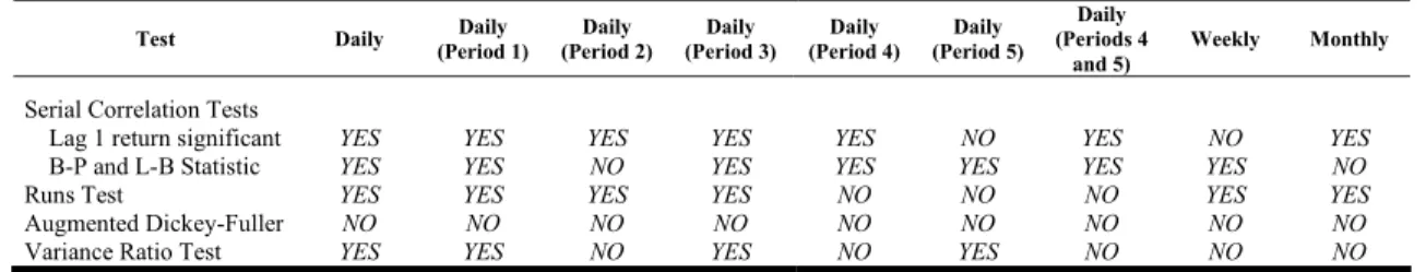
Table 6 summarizes the results of all the tests performed.
TABLE 6
Summary of Test Results: Random Walk Hypothesis Rejected?
Test Daily Daily
(Period 1) Daily (Period 2)
Daily (Period 3)
Daily (Period 4)
Daily (Period 5)
Daily (Periods 4
and 5)
Weekly Monthly
Serial Correlation Tests
Lag 1 return significant YES YES YES YES YES NO YES NO YES
B-P and L-B Statistic YES YES NO YES YES YES YES YES NO
Runs Test YES YES YES YES NO NO NO YES YES
Augmented Dickey-Fuller NO NO NO NO NO NO NO NO NO
Variance Ratio Test YES YES NO YES NO YES NO NO NO
Apart from the ADF test, which is very clearly favorable to the random walk hypothesis,
all other tests provide mixed evidence. Serial correlation is strong in daily returns, but tends to
reduce in weekly data and almost disappears in monthly data. The evidence is more favorable
to a random walk in periods 4 and 5, ranging from March 2000 to December 2006. None of
the results can be attributed to non-trading or infrequent trading, as the PSI-20 includes only
the 20 largest and most liquid shares.
All our findings confirm the previous results on the Portuguese market, namely Dias et
al. (2002) who find evidence against a random walk until 2001 and Worthington and Higgs
(2004) who state that Portugal satisfies the most stringent criteria for a random walk using
2000, the Portuguese stock market has become more weak-form efficient in recent years. This
is also corroborated by a clear decline of the dependence of daily returns on lagged returns, in
the same period.
References
Abraham, A., Seyyed, F. and Alsakran, S. “Testing the Random Behavior and Efficiency of the Gulf
Stock Markets” The Financial Review, 37, 3, 2002, pp. 469-480.
Dias, J., Lopes, L., Martins, V. and Benzinho, J.. “Efficiency Tests in the Iberian Stock Markets”,
2002, Available at SSRN: http://ssrn.com/abstract=599926.
Fama, E. “Efficient Capital Markets: A Review of Theory and Empirical Work” Journal of Finance,
25, 2, 1970, pp. 283-417.
Fama, E. and French, K. “Permanent and Temporary Components of Stock Prices” Journal of
Political Economy, 96, 2, 1988, pp. 246-273.
Gama, P. “A Eficiência Fraca do Mercado de Acções Português: Evidência do Teste aos Rácio de
Variância, da Investigação de Regularidades de Calendário e da Simulação de Regras de
Transacção Mecânicas”, Revista de Mercados e Activos Financeiros, 1, 1, pp. 5-28.
Grieb, T. and Reyes, M. “Random Walk Tests for Latin American Equity Indexes and Individual
Firms”, Journal of Financial Research, 22, 4, 1999, pp. 371-383.
Groenewold, N. and Ariff, M. “The Effects of De-Regulation on Share Market Efficiency in the
Asia-Pacific”, International Economic Journal, 12, 4, 1999, pp. 23-47.
Huang, B. “Do Asian Stock Markets Follow Random Walks? Evidence from the Variance Ratio Test”,
Applied Financial Economics, 5, 4, pp. 251-256.
Liu, C. and He, J. “A Variance-Ratio Test of Random Walks in Foreign Exchange Rates”, Journal of
Finance, 46, 2, p. 773-785.
Lo, A. and MacKinlay, A. “Stock Market Prices do not Follow Random Walks: Evidence from a
Ma, S. and Barnes, M. “Are China’s Stock Markets Really Weak-form Efficient?”, Centre for
International Economic Studies, Adelaide University, Discussion Paper 0119, May 2001.
MacKinnon, J. “Approximate Asymptotic Distribution Functions for Unit-Root and Cointegration
Tests”, Journal of Business & Economic Statistics, 12, 2, 1994, pp. 167-176.
Magnusson, M. and Wydick, B. “How Efficient are Africa’s Emerging Stock Markets”, Journal of
Development Studies, 38, 4, 2002, pp. 141-156.
Panas, E. “The Behaviour of Athens Stock Prices”, Applied Economics, 22, 12, 1990, pp. 1715-1727.
Smith, G., Jefferis, K. and Ryoo, H. “African Stock Markets: Multiple Variance Ratio Tests of
Random Walks”, Applied Financial Economics, 12, 4, 2002, pp. 475-484.
Smith, G. and Ryoo, H. “Variance Ratio Tests of the Random Walk Hypothesis for European
Emerging Stock Markets”, The European Journal of Finance, 9, 3, 2003, pp. 290-300.
Urrutia, J. “Tests of Random Walk and Market Efficiency for Latin American Emerging Markets”,
Journal of Financial Research, 18, 3, 1995, pp. 299-309.
Wheeler, F., Neale, B., Kowalski, T. and Letza S. “The Efficiency of the Warsaw Stock Exchange
Stock Exchange: The First Few Years 1991-1996”, The Poznan University of Economics Review,
2, 2, 2002, pp. 37-56.
Worthington, A. and Higgs, H. “Random Walks and Market Efficiency in European Equity Markets”,