Rev. Adm. Pública vol.51 número2

(1)

inequality in Brazil: an analysis of spending on education and

health from 1995 to 2012

Giovanni Pacelli Carvalho Lustosa da Costa

Universidade de Brasília / Programa de Pós-Graduação em Ciências Contábeis Brasília / DF — Brazil

Ivan Ricardo Gartner

Universidade de Brasília / Programa de Pós-Graduação em Administração Brasília / DF — Brazil

Income inequality is seen as a major problem of contemporary society. In order to reverse inequality the state can use allocation function in budgeting. his study sought to identify the impacts of allocation function in budgeting on income inequality for Brazilian states from 1995 to 2012. Spending on education and health was considered as an allocative function proxy, while the Gini coeicient, the heil coeicient, was used as a proxy for income inequality. his found the ratio between the richest 10% and the poorest 40%, and the ratio between the richest 20% and poorest 20%. he functional relationship between the two sets of variables was explored in the analysis of panel data and tobit regression. Considering aggregate expenditure on education and health of states and municipalities in the period, it was concluded that federative units that invested more in health have been better at reducing income inequality, with the opposite efect occurring for the cost of education. When spending on health and education are broken down into several sections, it can be seen that the federation units with higher volume of spending in the following sub-functions (2nd level of function) — Primary health care, hospital and outpatient care, prophylactic and therapeutic support and early childhood education — have made greater gains in reducing income inequality.

Keywords: regional economy; income inequality; Allocation function in budgeting; public spending on education and health.

O efeito da função orçamentária alocativa na redução da desigualdade de renda no Brasil: uma análise dos gastos em educação e saúde no período de 1995 a 2012

A desigualdade de renda é apontada como um dos grandes problemas da sociedade atual. A im de reverter o cenário desigual, o Estado pode atuar utilizando a função orçamentária alocativa. Este estudo buscou identiicar os impactos da função alocativa do orçamento sobre a desigualdade de renda, para as unidades federativas bra-sileiras no período de 1995 a 2012. Foram considerados como proxy da função alocativa os gastos com educação e saúde, enquanto foram utilizados como proxy da desigualdade de renda o coeiciente de Gini, o coeiciente de heil, a proporção entre os 10% mais ricos e os 40% mais pobres, e a proporção entre os 20% mais ricos e os 20% mais pobres. A relação funcional entre os dois conjuntos de variáveis foi explorada a partir da análise de dados em painel e da regressão tobit em painel. Considerando-se os gastos agregados em educação e saúde de estados e municípios no período, concluiu-se que as unidades da federação que investiram mais em saúde conseguiram reduzir as desigualdades de renda com maior intensidade, ocorrendo efeito oposto com as despesas com ensino. Quando os gastos em saúde e ensino foram desagregados em várias rubricas, concluiu-se que as unidades da federação com maior volume de gastos nas seguintes subfunções (2o_{nível da função):}_{atenção básica, assistência}

hospitalar, suporte proilático e ambulatorial, e educação infantil conseguiram reduzir as desigualdades de renda com maior intensidade.

Palavras-chave: economia regional; desigualdade de renda; função orçamentária alocativa; gastos públicos com educação e saúde.

DOI: http://dx.doi.org/10.1590/0034-7612155194

Article received on October 5, 2015 and accepted on October 27, 2016.

(2)

El efecto de la función asignativa en la reducción de la desigualdad de ingresos en Brasil: un análisis del gasto en educación y salud 1995-2012

La desigualdad de ingresos se ve como un problema importante de la sociedad contemporánea. Con el in de revertir la situación desigual, el Estado puede actuar mediante la función asignativa de presupuesto. Este estudio trata de identiicar los impactos de la función de la asignación de recursos del presupuesto en la desigualdad de ingresos para los estados de Brasil 1995 a 2012. Fueron considerados como un indicador de la función asig-nativa el gasto en educación y salud, mientras que se utilizaron como apoderado la desigualdad de ingresos el coeiciente de Gini, el coeiciente de heil, la relación entre el 10% más rico y el 40% más pobre, y la relación entre el 20% más rico y el 20% más pobre. La relación funcional entre los dos conjuntos de variables se exploró a partir del análisis de datos de panel y el panel de regresión Tobit. Teniendo en cuenta los gastos agregados sobre la educación y la salud de los estados y municipios en el período, se concluyó que las Unidades de la Federación que han invertido más en salud han logrado reducir la desigualdad de ingresos con mayor inten-sidad, que se producen efecto contrario con el costo de la educación. Cuando el gasto en salud y educación ha sido dividido en varias secciones, se concluyó que las unidades de la federación con mayor volumen de gasto en la siguientes subfunciones (segundo nivel de función): atención primaria, atención hospitalaria, asistencia preventiva y la atención ambulatoria, y educación de la primera infancia han logrado reducir la desigualdad de ingresos con mayor intensidad.

Palabras clave: economía regional; la desigualdad de ingresos; presupuesto función asignativa; el gasto público en educación y salud.

1. INTRODUCTION

he excessive income and wealth concentration separating social classes and increasing inequalities is one of the central problems of modern capitalism according to the Keynesian school of thou-ght. his imbalance hinders the maintenance of full employment in modern economies, because the small population of rich, who beneit from the income and wealth concentration, consume a smaller part of the total consumer goods when compared to what is consumed by the mass of poor population. he result is a weaker demand for consumer goods, which discourages its production and, indirectly, of capital goods. In addition, the excessive concentration of wealth jeopardizes the legitimacy of capitalism itself, because it creates social groups that enjoy social wealth without ha-ving contributed to its production (Keynes, 1996; Carvalho, 2008). he solution for this problem based on Keynesianism (adopted most oten by economists) lays mainly in the promotion of ins-titutional changes, such as the introduction of progressive taxes and capital gain taxes (especially on inheritance). he economic policy could help, but it would not be particularly strong to this end (Keynes, 1996; Carvalho, 2008).

Recently, in September 2000, 189 nations signed a pledge to ight extreme poverty and other issues in society. his promise was expressed by the 8 Millennium Development Goals (MDGs) that were to be achieved by 2015 (Millennium Development Goals, 2014). In September 2010, the world renewed its commitment to accelerate progress towards meeting these goals.

(3)

showed a very low development. On the other hand, the results show that inequalities persist within the metropolitan regions, even with the extraordinary progress made (Millennium Development Goals, 2014).

Regarding this negative result pointed out in the UN’s report, Paes and Siqueira (2008) had already warned that one of the great paradoxes of the present time is the coexistence of extremely developed economies amid enormous pockets of poverty. his happens both between countries on the same continent and between regions of the same country. he distribution of per capita

income in rich developed economies and in pockets of poverty seems to exhibit a persistent pat-tern: the two extremes seem to diverge from each other. he rich becoming richer and the poor becoming poorer.

As for the discussion on possible solutions to ight excessive income and wealth concentration, Musgrave and Musgrave (1980) proposed three economic functions of the modern budget: distribu-tion, which aims to adjust income distribution and the ofer of goods and services to the population in need; allocation, which aims to adjust allocation of resources; and the stabilization function, which aims to maintain economic stability.

Contemporary studies on inequality have as one of its references the work of Simon Kuznets:

Economic growth and income inequality (1955). Kuznets (1955) used a dual model with an agricultural and a non-agricultural sector — modern and dynamic — in order to analyze the relationship between income inequality and economic growth. he author’s indings indicate that income inequality would rise in the short term and, with economic growth, inequality would reduce forming an inverted U. hus, it was assumed that countries with a low degree of development would tend to present a higher level of income inequality in the short term and that this relationship would tend to revert as these countries work their way to achieve higher levels of per capita income.

Considering the conclusions of the Kuznets study, which focuses on the stabilization function related to economic growth, this work focuses only on the allocation and its relations with income inequality, the phenomenon that increases social problems.

Although they have not been organized in this way, previous works have used elements of the allocation function as independent variables.

Studies by Meltzer and Richard (1983), Perotti (1992), Easterly and Rebelo (1993), Lindert (1996), Perotti (1996), Partridge (1997), Gouveia and Masia (1998), Bassett, Burkett and Putterman (1999), Rodriguez (1999), Tanninen (1999), Castronova (2001), Jha, Biswal and Biswal (2001), Panizza (2002), Sylwester (2002), Mello and Tiongson (2006), Bergh and Fink (2008), Zhang (2008) and Holzner (2010) use public spending and elements of the allocation function in budgeting, as an attempt to evaluate their respective impact on reducing income inequality.

(4)

the inequality). Studies by Jha, Biswal and Biswal (2001) and Lima, Moreira and Souza (2013) used poverty indicators. he variation in the income index was used in the study by Lindert (1996). he asymmetric distribution was used in the study by Rodriguez (1999). Finally the per capita income, was used in the study by Castronova (2001).

Considering this context, the research question is: what is the efect of education and health spen-ding on reducing income inequality in the Brazilian States between 1995 and 2012?

herefore, this study aims to evaluate the reduction of income inequalities in Brazilian States from the iscal variables that are representative of the allocation function: spending on health and education.

his article is divided into ive sections. Ater this introduction, section 2 presents a review of the literature on income inequality and the economic functions of the budget. Section 3 presents aspects of the methodology adopted in this research such as the description of the variables and the econo-metric models used. Section 4 describes and analyzes the empirical results concerning the impact in terms of elasticity coeicients of factors that contribute to the reduction of income inequality using panel data analysis and the regression analysis tobit model with panel data. Finally, section 5 presents the conclusions of the study.

2. THEORETICAL FRAMEWORK

2.1 PERCEPTIONS OF INEQUALITY

Inequality is not a natural fact, but a social construction. It depends on circumstances and is largely the result of political choices made throughout the history of each society. All societies experience inequalities and they are presented in many diferent ways such as prestige, power, income. he origins of inequalities are as varied as the way they are expressed. he challenge is not only to describe the factors and elements of social inequalities, but also to explain how and why they remain or even increase in society, despite the modern values that push for equality (Scalon, 2011).

In this sense, the perception of inequality is relative when it comes to the objects of the analysis. Hypothetically, if an entire population lives in poverty and at the same level of poverty, then there is no inequality, but there is poverty. On the other hand, if rich people as well as very rich people form the population of a country, then there is no poverty but there is inequality. herefore, poverty can be reduced without changing the inequality.

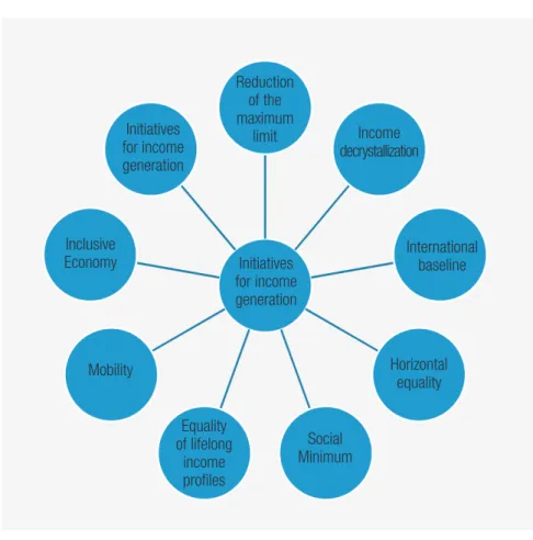
According to Cowell (2011), equality or inequality can be interpreted in diferent ways, which are described in Figure 1.

(5)

by a relatively disadvantaged group. he reduction of the maximum limit aims to limit the share of resources received by the most favored part of the population. he income and wealth decrystalli-zation aims to eliminate the disproportionate advantages in education, political power, and social acceptability that may be linked to an advantage (disadvantage) in income or wealth. he objective of the international baseline is that a given nation in analysis should not be more unequal than another comparable nation (Cowell, 2011).

FIGURE 1 PERSPECTIVES FOR INTERPRETATION OF INEQUALITY

Reduction of the maximum

limit Initiatives

for income generation

Inclusive Economy

Mobility

Equality of lifelong

income profiles

Social Minimum

Horizontal equality

International baseline Income

decrystallization

Initiatives for income generation

Source: Adapted from Cowell (2011).

In addition, Cowell (2011) incorporates additional elements to the measurement of inequality: (i) the speciication of the social unit of measure — individual, the nuclear family or the extended family; (ii) the description of the attribute of the dependent variable: income, wealth, land ownership, voting power, etc.; (iii) the method of representation or aggregation of income allocation among people in a given population.

(6)

2.2 ECONOMIC FUNCTIONS OF BUDGET

Keynesians argued that the government should intervene in the economy by way of iscal and monetary policies in order to promote full employment, price stability, and economic growth (Keynes, 1996).

To combat recession or depression, the government should increase its spending or reduce taxes, and this option would increase spending on private consumption. Also, the government should make more money available at lower interest rates in the expectation that this increases investment. As for controlling inlation caused by excessive aggregate spending, the government should reduce its own spending, raise taxes to reduce spending on private consumption or reduce the money supply to raise interest rates, which would curb excessive investment spending (Brue, 2005).

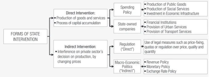
Figure 2 illustrates a detailed view of the forms of State intervention in the economy.

FIGURE 2 FORMS OF STATE INTERVENTION IN ECONOMY

FORMS OF STATE INTERVENTION

Direct Intervention:

• Production of goods and services • Process of capital accumulation

Indirect Intervention:

• Interference on private sector’s

decision on production, by changing prices

Spending Policy

State-owned companies

Regulation (“Direct”)

Macro-Economic Politics (“Indirect”)

• Production of Public Goods • Production of Social Services • Investment in Economic Infrastructure

• Financial Institutions • Provision of Urban Services • Provision of Transport Services

Use of legal measures such as price-fixing, quotas or regulation over price, quality and quantity

• Revenue Policy • Monetary Policy • Exchange Rate Policy

Source: Adpated from Rezende (2001).

As observed in Figure 2, the State can intervene in the economy directly and indirectly. Among the forms of direct intervention are the spending policy and state-owned companies (Rezende, 2001). In the spending policy, which is relected in the budget, the State acts as the main client of the internal market, whereas the State-owned companies act in strategic sectors of the industry.

Among the forms of indirect intervention, revenue and regulatory policies stand out (Rezende, 2001). Revenue policy, which is directly related to the tax system, comprises, among other measures, raising taxes or the waiver of revenues. As for regulation, the government works through its regulatory agencies to interfere in price, quality, and quantity of public concessions.

Following a similar line of State intervention in the economy, Musgrave and Musgrave (1980) established that it is the competency of the State to perform three typical functions: (i) allocation; (ii) distribution; and (iii) stabilization.

(7)

TABLE 1 ECONOMIC FUNCTIONS OF BUDGET

Function Characteristic

Allocation

It is comprised of provision of public goods, or process dividing the use of total resources of economy between public and private goods, as well as the process through which the composition of public goods is selected. Public goods cannot be offered as society needs by the market system. The fact that the benefits generated by public goods are available for all consumers implies no voluntary payment to suppliers of these goods. Thus, government is responsible to determine the type and quantity of public goods to be offered, as well as calculate the level of contribution for each consumer. In addition to the pure public goods, the State can provide semi-public goods such as education and health. These goods, despite being rivals and exclusives, and can be supplied by the market, present positive externalities that justify their provision or subsidy by the public sector.

Distribution

This function refers to income distribution, resulting from factors of production — capital, work and land — and selling of these factors’ services in the market. It can be applied by using transference mechanisms, progressive taxes and subsidies ensuring conformity with what society considers a fair distribution.

Stabilization

Relates to the use of budgetary policy with the aim of keeping full employment. This policy can be expressed directly, by the variation of public spending in consumption and investment; by the reduction of tax rates, which increases private sector’s disposable income.

Source: Musgrave and Musgrave (1980).

Based on the concept of economic functions of budget, the following variables were identiied: for allocation — spending on health and education; for distribution — progressive taxes and transfers of direct income; for stabilization — inlation and employment rate. his study focuses on the allocation function.

2.3 STATE OF THE ART ON THE ALLOCATION FUNCTION AND THE REDUCTION OF SOCIAL INEQUALITIES Several studies have sought to assess the efects of iscal variables on inequality. However, as explained in section 2.1, it is possible to analyze inequality on diferent perspectives, which brings a plurality of methods and dependent and independent variables to the discussion.

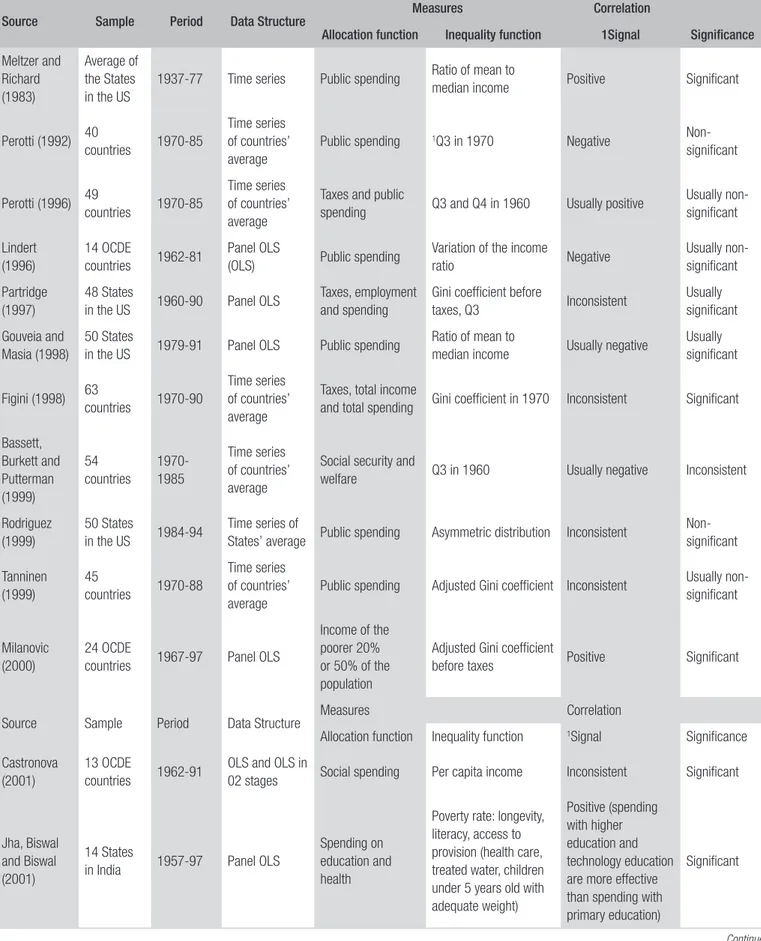
Table 2 presents the studies of researchers who sought to ind the relationship between the elements of the allocation function and income inequality. Meltzer and Richard (1983), Perotti (1992), Easterly and Rebelo (1993), Perotti (1996), Lindert (1996), Gouveia and Masia (1998), Bassett, Burkett, and Putterman (1999), Rodriguez (1999), Tanninen (1999), Castronova (2001), Jha, Biswal, and Biswal (2001), Sylwester (2002), Bergh and Fink (2008), Zhang (2008), Holzner (2010) as well as Araújo, Alves, and Bessaria(2013) used public spending and elements of the allocation function, in an attempt to assess their impact on the reduction of social inequalities.

(8)

Continue

TABLE 2 PREVIOUS STUDIES ON INEQUALITIES AND ALLOCATION FUNCTION

Source Sample Period Data Structure Measures Correlation

Allocation function Inequality function 1Signal Signiicance

Meltzer and Richard (1983)

Average of the States in the US

1937-77 Time series Public spending Ratio of mean to

median income Positive Significant

Perotti (1992) 40

countries 1970-85

Time series of countries’ average

Public spending 1_{Q3 in 1970} _Negative

Non-significant

Perotti (1996) 49

countries 1970-85

Taxes and public

spending Q3 and Q4 in 1960 Usually positive

Usually non-significant Lindert (1996) 14 OCDE countries 1962-81 Panel OLS

(OLS) Public spending

Variation of the income

ratio Negative Usually non-significant Partridge (1997) 48 States

in the US 1960-90 Panel OLS

Taxes, employment and spending

Gini coefficient before

taxes, Q3 Inconsistent

Usually significant

Gouveia and Masia (1998)

50 States

in the US 1979-91 Panel OLS Public spending

Ratio of mean to

median income Usually negative

Usually significant

Figini (1998) 63

countries 1970-90

Taxes, total income

and total spending Gini coefficient in 1970 Inconsistent Significant

Bassett, Burkett and Putterman (1999) 54 countries 1970-1985 Time series of countries’ average

Social security and

welfare Q3 in 1960 Usually negative Inconsistent

Rodriguez (1999)

50 States

in the US 1984-94

Time series of

States’ average Public spending Asymmetric distribution Inconsistent

Non-significant Tanninen (1999) 45 countries 1970-88 Time series of countries’ average

Public spending Adjusted Gini coefficient Inconsistent Usually non-significant

Milanovic (2000)

24 OCDE

countries 1967-97 Panel OLS

Income of the poorer 20% or 50% of the population

Adjusted Gini coefficient

before taxes Positive Significant

Source Sample Period Data Structure Measures Correlation

Allocation function Inequality function 1_Signal _Significance

Castronova (2001)

13 OCDE

countries 1962-91

OLS and OLS in

02 stages Social spending Per capita income Inconsistent Significant

Jha, Biswal and Biswal (2001)

14 States

in India 1957-97 Panel OLS

Spending on education and health

Poverty rate: longevity, literacy, access to provision (health care, treated water, children under 5 years old with adequate weight)

Positive (spending with higher education and technology education are more effective than spending with primary education)

(9)

Source Sample Period Data Structure

Measures Correlation

Allocation function Inequality function 1Signal Signiicance

Panizza (2002)

46 States

in the US 1970-80

Time series of States’ average

Taxes, progressive taxes and public spending

Q3 in 1970 Usually positive Inconsistent

Sylwester (2002)

50

Spending on

education Gini coefficient Negative Significant

Mello and Tiongson (2006)

Between 49 and 55 countries

1972-98, and 1970-98

Panel OLS e panel tobit

Spending on social security (health included) and welfare (percentage of GDP); Transfers (percentage of GDP)

Gini coefficient, per capita income, percentage of the population over 65 years old, democracy index Negative Usually significant Bergh and Fink (2008) 35 countries

1980-2000 Panel OLS

Spending on education

Gini coefficient

Positive Significant

Zhang (2008) 50

Spending on education, separated in secondary and high education

Gini coefficient

Negative for secondary education and positive for higher education Significant Holzner (2010) 28 countries from Central, East and Southeast Europe 1989-2006 Generalized

least squares Spending

Gini coefficient

Spending with social protection and health were negatively related Significant Araújo, Alves and Bessaria (2013) Brazilian States 2004-09 Panel fixed effects Spending on education, health care and the federal conditional cash transfer program (Bolsa Família)

Number of people in households with per capita household income below the line of extreme poverty; Number of people in households with per capita income below the line of poverty; Gini coefficient and Theil-T coefficient Negatively related Significant only for poverty indicators

Source: Elaborated by the Authors

Note:1_{Q3 — proportion of the income obtained by the 3}o_{quintile of the population. Larger the proportion, smaller the inequality.}

(10)

Continue

From the results found in previous studies and considering the theory, the central hypothesis of this research is established as follows: the States of Brazil that present a higher volume of spending on education and health reduced income inequality, ceteris paribus.

he choice for the States spending on education and health was made because these areas that lead to positive externalities by reducing income inequality in line with the social minimum, inclusive economy, and decrystallization of wealth, considering the above in Figure 1 of section 2.1.

In order to expand the possibilities of the study, the element of royalties was included. Studies by Sousa, Cribari-Neto and Stosic (2005) identiied that the Brazilian municipalities that receive substantial royalties tend to be less eicient, then suggesting that extra revenue, instead of en-couraging full use of resources, contributes to the relaxation of iscal constraints and increased ineiciency.

3. METHODOLOGY OF EMPIRICAL ANALYSIS

his section will present the techniques used for quantitative data analysis, as well as detailing the functional models, econometric models and variables that serve as proxies to test the research hypo-thesis stated in the previous section.

3.1 SAMPLING

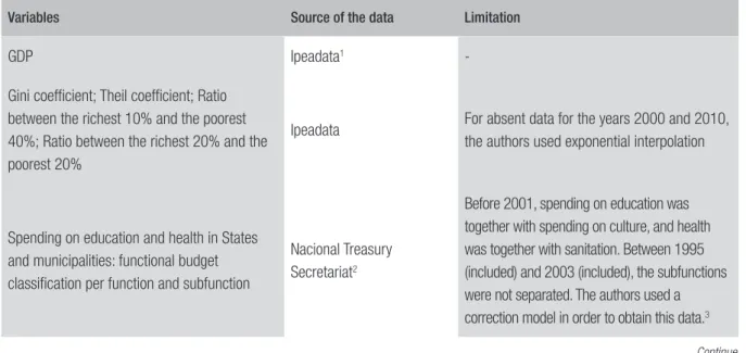
he population in this study is made up of all of the Brazilian States. he data was collected for each of the 18 years referring to the period from 1995 to 2012, of the 26 Brazilian States, including the Federal District. Table 3 contains the variables and sources of data.

TABLE 3 VARIABLES, SOURCES OF DATA AND LIMITATIONS

Variables Source of the data Limitation

GDP Ipeadata1

-Gini coefficient; Theil coefficient; Ratio between the richest 10% and the poorest 40%; Ratio between the richest 20% and the poorest 20%

Ipeadata For absent data for the years 2000 and 2010, the authors used exponential interpolation

Spending on education and health in States and municipalities: functional budget classification per function and subfunction

Nacional Treasury Secretariat2

(11)

Variables Source of the data Limitation

Revenues from oil royalties

Brazilian National Agency of Petroleum, Natural Gas and Biofuels4

Absent data for 1995 and 1996

Revenues from royalties paid by the electricity sector

Brazilian Electricity

Regulatory Agency5 Absent data for 1995 and 1996

Source: Elaborated by the authors 1_{Available at: <www.ipeadata.gov.br/>.}

2_{Available at: <www.tesouro.fazenda.gov.br/pt/contas-anuais>.}

3_{In the case of spending on health and education, it was considered the mean in each State: the sum of the expenses on health between} 2004 and 2012 was divided by the sum of the expenses on health and sanitation between 2004 and 2012. he result was multiplied by the amount of expenses on health and sanitation, year by year, from 1995 to 2003.

4_{Data was provided by the system E-SIC: <www.acessoainformacao.gov.br/sistema/site/index.html?ReturnUrl=%2fsistema%2f>, protocol} 48700006560201500 of August 31st 2015.

5_{Available at: <www.aneel.gov.br/aplicacoes/cmpf/gerencial/>.}

he year 1995 was the irst year of the “Real”, an economic plan that generated credit stability and provided family planning (which may have also contributed to the reduction of income inequality during the study period). However, this phenomenon will not be explored.

3.2 THE PROPOSED MODEL AND RESEARCH VARIABLES

The study of Lundberg and Squire (2003) uses equation 1 as a reference.

it it

it

S

Z

e

Gini

=

α

+

´

ϖ

+

´

ψ

+

(1)

he equation states that inequality “Gini” of a country in a region or country “i” at a period “t” is a function of variables related to the vector of economic growth and inequalities (S_it) and of the vector of variables related with the vector of inequalities without relation to economic growth (Zit).

From the adjusted previous functional model and considering the research hypothesis: the States of Brazil that present higher volume of spending on education and health reduced income inequality, ceteris paribus; the functional model was provided as in equation 2.

        = t i s t i t i s t i j t i PIB DSAU PIB DEDU f DES , , , , , , ,

, ; (2)

Where the income inequality index (DES) in a certain State “i” is a function of percentage ex-penditures on education (DEDU) and health (DSAU) of a certain public entity “i” in a determined period “t”. he “j” attribute identiies diferent variables to measure income inequality. he “s” attribute identiies the aggregation of expenditures that one wishes to highlight. he econometric model in equation 3 is presented as follows.

(12)

Considering the index DES, income inequality, of a given State “i” is a function of percentage expenditure on education and health of this State in a given period “t”. he “j” attribute identiies the diferent variables of inequality: the Gini coeicient, the heil coeicient, the ratio between the richest 10% and poorest 40%, the ratio between the richest 20% and poorest 20%. he “s” attribute identiies whether the expenses in question are: only State, only municipal, or State and municipal consolidated.

he “RNE” dummy variable identiies the States of the Northeast, the “RCO” dummy variable identiies the States of the Midwest, the “RSE” dummy variable identiies the States of the Southeast, the “RSU” dummy variable identiies the States of the South.

he “Royp” variable contains the amounts received from oil royalties by States and municipalities and the variable “Royse” refers to royalties received from the electricity sector by States and munici-palities. Table 4 provides a breakdown of variables.

Both the functional model and the econometric model only consider variables of allocation function such as health and education. hey do not consider progressive taxes or transfers of income directly related to the distribution function.

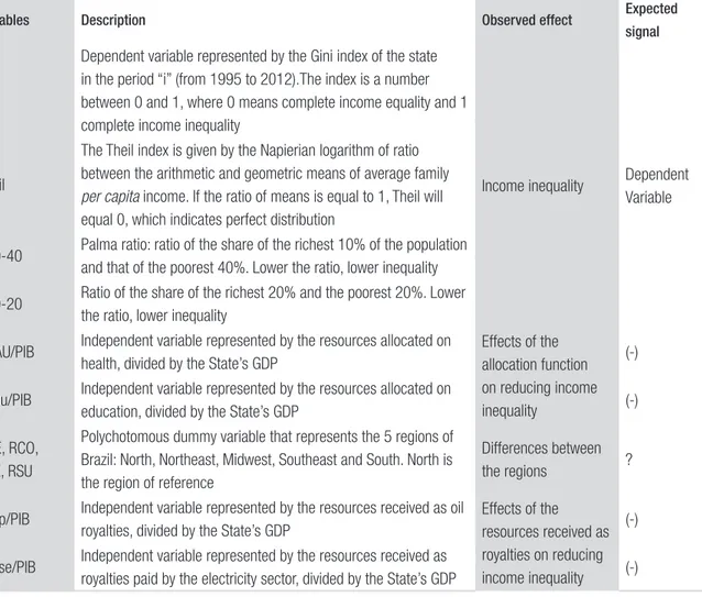
TABLE 4 VARIABLES DESCRIPTION AND EXPECTED SIGNAL

Variables Description Observed effect Expected signal

Gini

Dependent variable represented by the Gini index of the state in the period “i” (from 1995 to 2012).The index is a number between 0 and 1, where 0 means complete income equality and 1 complete income inequality

Income inequality Dependent Variable Theil

The Theil index is given by the Napierian logarithm of ratio between the arithmetic and geometric means of average family

per capita income. If the ratio of means is equal to 1, Theil will

equal 0, which indicates perfect distribution

P10-40 Palma ratio: ratio of the share of the richest 10% of the population and that of the poorest 40%. Lower the ratio, lower inequality

P20-20 Ratio of the share of the richest 20% and the poorest 20%. Lower the ratio, lower inequality

DSAU/PIB Independent variable represented by the resources allocated on health, divided by the State’s GDP

Effects of the allocation function on reducing income inequality

(-)

Dedu/PIB Independent variable represented by the resources allocated on

education, divided by the State’s GDP (-)

RNE, RCO, RSE, RSU

Polychotomous dummy variable that represents the 5 regions of Brazil: North, Northeast, Midwest, Southeast and South. North is the region of reference

Differences between

the regions ?

Royp/PIB Independent variable represented by the resources received as oil royalties, divided by the State’s GDP

Effects of the resources received as royalties on reducing income inequality

(-)

Royse/PIB Independent variable represented by the resources received as

royalties paid by the electricity sector, divided by the State’s GDP (-)

(13)

Spending on education and health generate positive externalities and can contribute to the re-duction of income inequality in the perspectives of the social minimum, inclusive economy and the decrystallization of wealth. herefore, the tendency is that the larger the amount of resources, the lower the income inequality is (Cowell, 2011; Giacomoni, 2012).

he Federal Constitution of Brazil from 1988 establishes that education and health are social rights guaranteed to all citizens.1

Education and health, when well distributed and ofered with equality, tend to ensure the social minimum because they ensure that everyone has a minimum standard of wellbeing; reduce the fe-eling of exclusion from society caused by diferences in income; and because they aim to eliminate the disproportionate advantages in education (Cowell, 2011).

hose who receive substantial income from royalties tend to have more resources to allocate for education and health; therefore, they would be more likely to reduce income inequality.

3.3 METHODS TO EVALUATE THE PROPOSED MODEL

he econometric model proposed in equation (3) was analyzed according to the panel data analysis with ixed efects and the tobit regression on panel data. he tobit regression on panel data was con-ducted with the aim of testing whether the speciication of the truncated dependent variable would have a better performance. hus, the intention is to validate the results through using two distinct approaches.

Panel data analysis with ixed efects is more appropriate when the units of observation in the sample are the entire population. In addition, it requires that the intercept in the regression model is diferent for the observation units (i), but not over time (t); and that all estimates of slope coeicients are ixed for observation units (i) and time (t) (Baltagi, 2005).

he tobit panel has the following characteristics: (i) the model is linear; (ii) the dependent varia-ble is continuous and censored in the range between 0 and 1. he fact that the dependent variavaria-ble is censored indicates that the estimation of parameters by Ordinary Least Squares is not appropriate, which justiies the use of the tobit model. In the tobit model the parameters are estimated by maxi-mum likelihood; (iii) the model combines the observation units (States) over time; (iv) it is evident that there is heterogeneity between the States, justifying the existence of panel data (Baltagi, 2005).

Considering the features of the dependent variables, the OLS ixed efects tend to be more suitable for the dependent variables P10-40 and P20-20, while the tobit panel tends to be more suitable for the Gini and heil dependent variables.

4. RESULTS AND ANALYSIS

his section presents the research results. Subsection 4.1 presents descriptive data of the research’s main variables. In subsection 4.2, spending is presented by function: health and education, whereas in subsection 4.3 spending is presented by subfunction (second level of function). his measure for section 4.3 was necessary from the results obtained in section 4.2.

(14)

4.1 DESCRIPTIVE DATA FROM THE MAIN VARIABLES USED

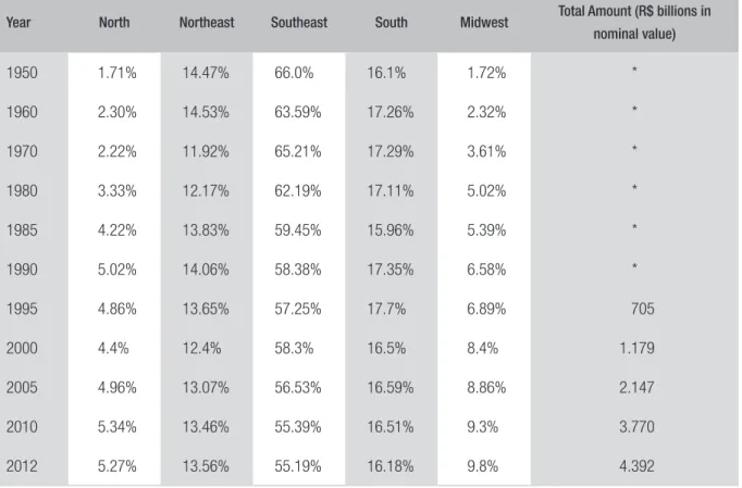
TABLE 5 PARTICIPATION OF BRAZILIAN REGIONS IN NATIONAL GDP

Year North Northeast Southeast South Midwest Total Amount (R$ billions in nominal value)

1950 1.71% 14.47% 66.0% 16.1% 1.72% *

1960 2.30% 14.53% 63.59% 17.26% 2.32% *

1970 2.22% 11.92% 65.21% 17.29% 3.61% *

1980 3.33% 12.17% 62.19% 17.11% 5.02% *

1985 4.22% 13.83% 59.45% 15.96% 5.39% *

1990 5.02% 14.06% 58.38% 17.35% 6.58% *

1995 4.86% 13.65% 57.25% 17.7% 6.89% 705

2000 4.4% 12.4% 58.3% 16.5% 8.4% 1.179

2005 4.96% 13.07% 56.53% 16.59% 8.86% 2.147

2010 5.34% 13.46% 55.39% 16.51% 9.3% 3.770

2012 5.27% 13.56% 55.19% 16.18% 9.8% 4.392

Sources: IBGE2_{(2015) and Ipeadata (2015).}

Note: * it was not considered due to the changes in the currency.

It is possible to observe that in 1950, around 82% of the wealth was concentrated in the South and Southeast regions, whereas in 2010, this percentage dropped to 72%. In 60 years, there was a redistri-bution of only 10% in wealth generation. An important factor is that in absolute terms, the GDP in the Northeast region, went from R$ 84 billion in 1995 to R$ 508 billion in 2010, an increase of 600%. In the Southeast, GDP went from R$ 417 billion in 1995 to R$ 2.088 billion in 2010, an increase of 500%. herefore, it is important to recognize that there was an incremental increase in the generation of wealth in all regions, even though the concentration in the Southeast persists.

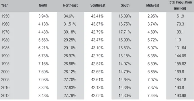
Table 6 below presents data about the population.

(15)

TABLE 6 POPULATION IN BRAZILIAN REGIONS

Year North Northeast Southeast South Midwest Total Population (million)

1950 3.94% 34.6% 43.41% 15.09% 2.95% 51.9

1960 4.13% 31.51% 43.87% 16.75% 3.74% 70.3

1970 4.43% 30.18% 42.79% 17.71% 4.89% 93.1

1980 5.56% 29.25% 43.47% 15.99% 5.72% 119

1985 6.21% 29.10% 43.10% 15.53% 6.07% 131.64

1990 6.73% 28.97% 42.79% 15.15% 6.36% 144.09

1995 7.16% 28.86% 42.54% 14.97% 6.59% 155.82

2000 7.60% 28.12% 42.65% 14.79% 6.85% 169.8

2005 7.98% 27.70% 42.61% 14.64% 7.07% 184.18

2010 8.32% 27.83% 42.13% 14.36% 7.37% 190.8

2012 8.43% 27.79% 42.05% 14.30% 7.44% 193.98

Sources: Datasus (2015) and Ipeadata (2015).

When comparing the proportion of population distribution in table 6 with the proportion of wealth in table 5, it is possible to observe that one of the most disadvantaged regions — in terms of percentage — is the Northeast.

Tables 7 and 8 present indicators of income inequality in Brazilian regions.

TABLE 7 EVOLUTION OF GINI COEFFICIENT IN BRAZILIAN REGIONS

Year North Northeast Southeast South Midwest

1979 0.530 0.557 0.557 0.564 0.561

1985 0.549 0.595 0.567 0.561 0.587

1990 0.583 0.626 0.577 0.577 0.611

1995 0.584 0.604 0.567 0.565 0.585

1999 0.565 0.605 0.559 0.562 0.593

2005 0.530 0.571 0.543 0.515 0.577

2009 0.522 0.558 0.511 0.491 0.560

2012 0.513 0.542 0.505 0.468 0.531

(16)

TABLE 8 EVOLUTION OF THEIL-T COEFFICIENT IN BRAZILIAN REGIONS

1979 0.557 0.691 0.622 0.665 0.617

1985 0.622 0.807 0.638 0.644 0.708

1990 0.722 0.881 0.676 0.660 0.777

1995 0.713 0.810 0.645 0.645 0.689

1999 0.639 0.801 0.620 0.627 0.736

2005 0.577 0.705 0.594 0.523 0.712

2009 0.554 0.666 0.527 0.479 0.664

2012 0.529 0.676 0.551 0.450 0.599

Source: Ipeadata (2015).

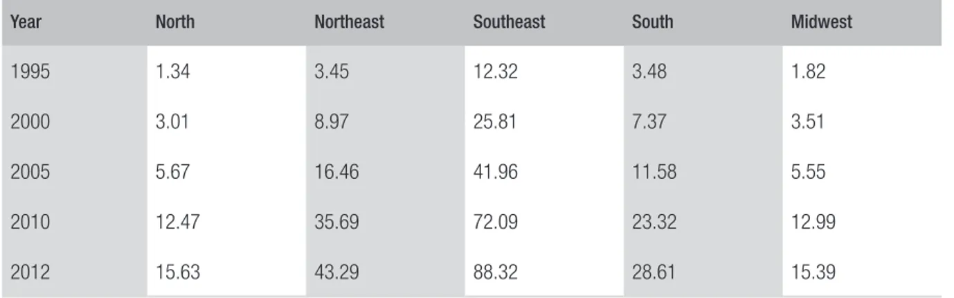
During the period from 1995 and 2012 the indicators of income inequalities improved. he South is the least and the Northeast the most unequal regions. Tables 9 and 10 show nominal values of State and municipal spending separated by regions, in the period covered by this study.

TABLE 9 EVOLUTION OF THE SPENDING ON EDUCATION — STATE AND MUNICIPAL SPENDING —

NOMINAL VALUES IN R$ BILLIONS

1995 1.34 3.45 12.32 3.48 1.82

2000 3.01 8.97 25.81 7.37 3.51

2005 5.67 16.46 41.96 11.58 5.55

2010 12.47 35.69 72.09 23.32 12.99

2012 15.63 43.29 88.32 28.61 15.39

(17)

Continue

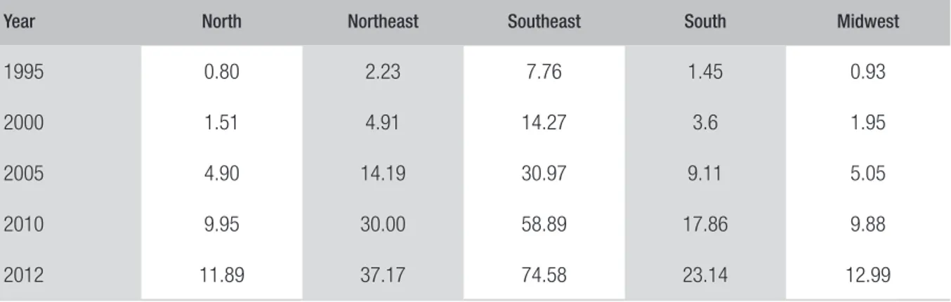
TABLE 10 EVOLUTION OF THE SPENDING ON HEALTH — STATE AND MUNICIPAL SPENDING —

NOMINAL VALUES IN R$ BILLIONS

1995 0.80 2.23 7.76 1.45 0.93

2000 1.51 4.91 14.27 3.6 1.95

2005 4.90 14.19 30.97 9.11 5.05

2010 9.95 30.00 58.89 17.86 9.88

2012 11.89 37.17 74.58 23.14 12.99

Source: Ipeadata (2015).

he Southeast has the largest amount of resources allocated to education and health, followed by the Northeast.

4.2 EVALUATION OF SPENDING PER FUNCTION

he results are presented considering 3 statistical methods: (i) panel data analysis; (ii) panel data analysis with ixed efects, (iii) tobit panel data. 03 tables are presented for each method: (i) State spending, (ii) municipal spending broken down by state, (iii) state and municipal spending broken down by state.

Tables 11, 12 and 13 show the tests results using panel data analysis.

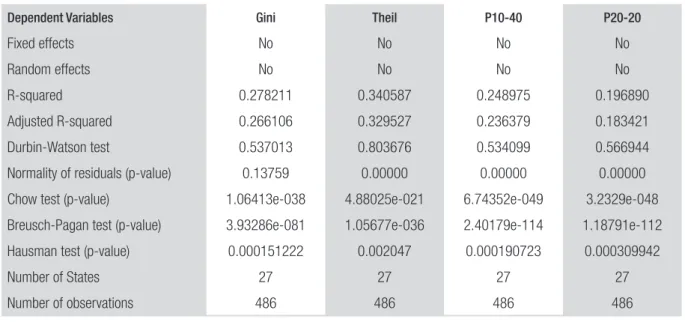
TABLE 11 RESULTS OF PANEL DATA ANALYSIS: STATE SPENDING

Dependent Variables Gini Theil P10-40 P20-20

Constant 0.557231*** 0.648005*** 18.1708*** 19.9547***

DSAU/PIB −0.861057*** −2.51383*** −73.6670*** −62.2865**

Dedu/PIB 0.327670*** 0.815862*** 33.6083*** 35.1267***

RNE 0.0322555*** 0.119373*** 3.34773*** 3.02151***

RCO 0.00669244 0.00531743 1.39167** 1.51587*

SER −0.00816456 −0.0297818 −0.792370 −1.01775

RSU −0.0377572*** −0.108434*** −2.98168*** −2.80039***

Royp −1.37777 −6.66002** −221.108** −311.268**

(18)

Dependent Variables Gini Theil P10-40 P20-20

Fixed effects No No No No

Random effects No No No No

R-squared 0.278211 0.340587 0.248975 0.196890

Adjusted R-squared 0.266106 0.329527 0.236379 0.183421

Durbin-Watson test 0.537013 0.803676 0.534099 0.566944

Normality of residuals (p-value) 0.13759 0.00000 0.00000 0.00000

Chow test (p-value) 1.06413e-038 4.88025e-021 6.74352e-049 3.2329e-048

Breusch-Pagan test (p-value) 3.93286e-081 1.05677e-036 2.40179e-114 1.18791e-112

Hausman test (p-value) 0.000151222 0.002047 0.000190723 0.000309942

Number of States 27 27 27 27

Number of observations 486 486 486 486

Source: Elaborated by the authors.

Note: ***Signiicant to 1%; **Signiicant to 5%; *Signiicant to 10%.

TABLE 12 RESULTS OF PANEL DATA ANALYSIS: MUNICIPAL SPENDING

Variables Gini Theil P10-40 P20-20

Constant 0.564414*** 0.629453*** 19.8008*** 22.1233***

DSAU/PIB −3.24996*** −8.36520*** −360.445*** −432.942*** Dedu/PIB 1.44029*** 4.87553*** 147.592*** 193.594***

RNE 0.0559801*** 0.171950*** 5.90264*** 5.70446***

RCO 0.0160185*** 0.0458700*** 1.97206*** 1.98641***

RSE 0.00173748 0.0101212 −0.169669 −0.597139

RSU −0.0327243*** −0.0775846*** −2.94343*** −3.04654*** Royp −1.72736** −7.59521*** −245.021*** −317.034***

Royse 3.87458 17.6831 −187.318 −949.273*

R-squared 0.422755 0.413631 0.429152 0.377689

Chow test (p-value) 0.000714581 2.8859e-020 3.68032e-040 3.4422e-039

(19)

TABLE 13 RESULTS OF PANEL DATA ANALYSIS: STATE AND MUNICIPAL SPENDING

Constant 0.575969 *** 0.673872*** 20.6867*** 22.9968***

DSAU/PIB −1.19773*** −2.81451*** −127.867*** −137.282***

Dedu/PIB 0.368970*** 0.926702*** 39.4913*** 44.4418***

RNE 0.0381549*** 0.138783*** 3.78629*** 3.32858***

RCO 0.000697084 0.00197931 0.432325 0.259102

SER −0.0148291** −0.0333564** −1.87158*** −2.44677***

RSU −0.0470369*** −0.117858*** −4.34633*** −4.53758***

Royp −0.980718 −6.03399** −165.616* −238.241**

Royse −1.26587 9.92894 −849.142* −1723.97***

R-squared 0.363055 0.386996 0.340358 0.276668

Chow test (p-value) 1.08765e-038 6.4103e-022 5.56765e-051 5.29794e-050

It is possible to observe in table 11 that the larger the proportion of spending on health on the GDP, the higher the tendency to reduce income inequality. his result is similar with the result shown by Jha, Biswal and Biswal (2001) and Holzner (2010), and with the assumptions from Cowell (2011) and Giacomoni (2012).

he idea is the same for the proportion of oil royalties and the royalties payed by the electricity sector. he regional efect was signiicant in the regions Northeast and South in comparison to the North. hese results are valid for the 4 indicators of income inequality selected in the research.

(20)

pooled model. Regarding Hausman test, it is observed that the panel data with ixed efects would be preferred over the panel data with random efects.

In table 12, which considers the municipal spending on education and health broken down by State, the results were similar to the ones in table 5. he diferences are: the regional efect became signiicant in the Midwest region; the panel data with ixed efects is still preferred for the dependent variable heil, whereas the panel data with random efect is preferred for the variables: Gini, P10-40 (ratio between the richest 10% and the poorest 40%) and P20-20 (ration between the richest 20% and the poorest 20%).

In table 13, which considers State and municipal spending separated on spending on education and health, the results were similar of those in table 5. he diferences found are: the regional efect became signiicant in the Southeast; the panel data with ixed efects is still the preferred for the va-riables Gini and heil, whereas the panel with random efects is preferred for the vava-riables P10-40 (ratio between the richest 10% and the poorest 40%) and P20-20 (ratio between the richest 20% and the poorest 20%).

In tables 11, 12 and 13 it is observed a high level of agreement regarding the signals of the inde-pendent and the deinde-pendent variables.

Tables 14, 15 and 16 present the results of the tests using OLS — ixed efects. It is important to clarify that it is not possible to use regional dummies in this method.

TABLE 14 RESULTS OF PANEL DATA ANALYSIS WITH FIXED EFFECTS: STATE SPENDING

Constant 0.592726*** 0.735866 *** 22.2565*** 24.4729***

DSAU/PIB −2.20860*** −5.26054 *** −234.328*** −262.643***

Dedu/PIB 0.340259*** 0.847441*** 37.4276*** 39.5296***

Royp −3.72202*** −8.72846** −426.184*** −408.912***

Royse −9.07689 −36.0064* −1150.30* −1364.84*

Fixed effects Yes Yes Yes Yes

R-squared LSDV 0.579131 0.531235 0.607876 0.577571

Joint test on designated regressors (p-value) 1.74095e-027 6.23714e-018 1.07511e-029 4.4491e-025

Test to differ groups intercepts (p-value) 9.23604e-065 2.03079e-056 3.12146e-070 1.02035e-061

(21)

TABLE 15 RESULTS OF PANEL DATA ANALYSIS WITH FIXED EFFECTS: MUNICIPAL SPENDING

Constant 0.595625*** 0.740833**** 22.8158*** 24.6266***

DSAU/PIB −3.48849*** −9.52842*** −376.607*** −462.995***

Dedu/PIB 1.12573*** 3.74239*** 114.476*** 177.321***

Royp −1.44971 −3.16433 −165.24 −133.541

Royse −3.68855 −20.0668 −502.433 −605.605

Fixed effects Sim Sim Sim Sim

Random effects Não Não Não Não

R-squared LSDV 0.632069 0.579179 0.671934 0.638438

Source: Elaborated by the authors.

TABLE 16 RESULTS OF PANEL DATA ANALYSIS WITH FIXED EFFECTS: STATE AND MUNICIPAL SPENDING

Constant 0.603123*** 0.761642*** 23.4786*** 25.7469***

DSAU/PIB −1.52046 *** −3.72834*** −165.166*** −183.620***

Dedu/PIB 0.229978*** 0.617514*** 25.4159*** 27.8046***

Royp −2.01167* −4.49039 −237.276** −198.135

Royse −3.36522 −21.2346 −496.564 −645.774

Fixed effects Sim Sim Sim Sim

Random effects Não Não Não Não

R-squared LSDV 0.628507 0.568643 0.663121 0.626674

(22)

In tables 14, 15 and 16, it is noted that the larger the proportion of spending on health on the GDP, the higher the tendency of reducing income inequality. Once more, the controversial result related to spending on education is repeated. his demands a deeper analysis starting from the expenditures break down.

he expected signal of the independent variables related to the royalties was in agreement in the 03 tables, even though they are not always statistically signiicant. his result conirms the previous assumption that the Brazilian territories that present a larger proportion of royalties on the GDP tend to reduce inequality more intensively.

Tables 17, 18 and 19 present the results of tests using tobit panel.

TABLE 17 RESULTS OF TOBIT PAINEL: STATE SPENDING

Constant 0.557231*** 0.648419*** 18.1708*** 19.9547***

DSAU/PIB −0.861057*** −2.54981*** −73.6670*** −62.2865**

Dedu/PIB 0.327670*** 0.827750*** 33.6083*** 35.1267***

RNE 0.0322555*** 0.117022*** 3.34773*** 3.02151***

RCO 0.00669244 0.00502309 1.39167** 1.51587*

SER −0.00816456 −0.0304459* −0.792370 −1.01775

RSU −0.0377572*** −0.108842*** −2.98168 *** −2.80039***

Royp −1.37777 −6.38195** −221.108** −311.268**

Royse −5.86680 −1.04253 −1325.64*** −2219.73***

Normality of residuals (p-value) 0.18012 0.00601954 1.86671e-009 1.4784e-022

TABLE 18 RESULTS OF TOBIT PANEL: MUNICIPAL SPENDING

Constant 0.564414*** 0.629453*** 19.8008*** 22.1233***

DSAU/PIB −3.24996*** −8.36520*** −360.445*** −432.942***

Dedu/PIB 1.44029*** 4.87553*** 147.592*** 193.594***

RNE 0.0559801*** 0.171950*** 5.90264*** 5.70446***

RCO 0.0160185*** 0.0458700 *** 1.97206*** 1.98641***

SER 0.00173748 0.0101212 −0.169669 −0.597139

RSU −0.0327243*** −0.0775846*** −2.94343*** −3.04654***

Royp −1.72736** −7.59521*** −245.021*** −317.034***

Royse 3.87458 17.6831 −187.318 −949.273*

(23)

Normality of residuals (p-value) 8.50279e-005 0.0297881 0.0100489 3.5735e-008

TABLE 19 RESULTS OF TOBIT PANEL: STATE AND MUNICIPAL SPENDING

Constant 0.575969*** 0.673872*** 20.6867*** 22.9968***

DSAU/PIB −1.19773*** −2.81451*** −127.867*** −137.282***

Dedu/PIB 0.368970*** 0.926702*** 39.4913*** 44.4418***

RNE 0.0381549*** 0.138783*** 3.78629*** 3.32858 ***

RCO 0.000697084 0.00197931 0.432325 0.259102

SER −0.0148291*** −0.0333564** −1.87158*** −2.44677***

RSU −0.0470369*** −0.117858 *** −4.34633*** −4.53758***

Royp −0.980718 −6.03399** −165.616* −238.241**

Royse −1.26587 9.92894 −849.142* −1723.97***

he results in the 3 tables above reinforce the results obtained in the previous tests pointing out that the larger the proportion of spending on health on the GDP, the higher the tendency of reducing income inequality. In the same way, there is a repetition of the same controversial result related to spending on education.

his result in education contradicts the result found by Jha, Biswal and Biswal (2001), Sylwester (2002), Mello and Tiongson (2006), Bergh and Fink (2008) and Zhang (2008). he result also con-tradicts the assumptions from Cowell (2001) and Giacomoni (2012).

In comparison to the model of the USA that emphasizes the primary and secondary education in allocating State’s resources, granting to the private sector the most part of the initiative and responsibility when it comes to higher education, it is possible to observe that in Brazil the private sector competes with the State since primary education. hus, whilst in the United States the majority of the population (of all social classes) attend public schools for primary and secondary education, in Brazil a considera-ble part of the population is attending primary and secondary education ofered by the private sector.

(24)

Continue

4.3 EVALUATION OF SPENDING BY SUBFUNCTION

Considering the results in the previous subsection, it is necessary to separate spending on education and on health in subfunctions. herefore, the econometric model in equation 3 showing the spen-ding functions education and health was broken down as presented in equation 4, by subfunctions of spending on health and education.

(4)

As for the function of health, the variable “AtBas” represents spending on the subfunction primary health care. “AssHosp” means the spending on the subfunction hospital and outpatient care. “Suproilat” means the spending on the subfunction prophylactic and therapeutic support. “VigSan” is the spending on the subfunction health surveillance. “VigEpi” is the spending on the subfunction “epidemiological surveillance”. “Ali” is the spending on the subfunction food and nutrition. Finally, “OutrasSau” represents the spending on the subfunction “other expenditures on health”. Regarding the function education, the variable “Fund” represents the spending on the subfunction primary education. “Medio” is the spending on the subfunction secondary education. he variable “Ensprof ” represents the spending on professional education. he variable “Supe” the spending on the subfunction higher education. “Infantil” is the spending on the subfunction early childhood education. “EJA”, the spending on adults’ and young adults’ education. “Especial” represents the spending on the subfunction special education. Finally, “OutrasEdu” represents the spending on the subfunction other expenditures on education. Other variables were presented in equation 3.

Tables 20, 21 and 22 show the results of the tests using tobit panel.

TABLE 20 RESULTS OF TOBIT PANEL: STATE SPENDING PER SUBFUNCTION

Dependent variables Gini Theil P10-40 P20-20

Constant 0.567239*** 0.680828*** 19.3773*** 21.2566*** Primary health care/GDP −0.397113 −2.20166 30.5719 123.415

Hospital care/GDP −0.280921 −1.01464* −13.7024 −4.99535 Prophylactic support/GDP −5.52664*** −18.3998*** −658.870*** −745.539***

Health surveillance/GDP 5.22978*** 11.7557** 518.522*** 496.918** Epidemiological surveillance/ GDP −10.3132 −46.3498* −898.952 −541.118

(25)

Continue

Other expenditures on health/GDP −1.13523*** −2.60327** −88.3343** −86.2024*

Primary education/GDP 0.0579263 −0.0263398 −3.34866 −3.42524 Secondary education/GDP −0.0354357 −1.44602 −10.5688 59.5368

Professional education/GDP −3.15187 −10.8978 −269.861 −356.995 Higher education/GDP −0.489651 −0.431533 5.12441 −35.4990

Early childhood education/GDP 11.9802** 13.8384 1629.09*** 1980.32***

Adults’ and young adults’ education/GDP −3.97810 −14.9639 −517.383 −808.547

Special education/GDP 3.35274 6.49415 483.347 310.804 Other expenditures on education/GDP 0.185691 1.44529 ** 6.71220 1.74036

RNE 0.0289955*** 0.109902*** 3.02599*** 2.49557***

RCO 4.78443e-05 −0.0169527 0.607162 0.695667

SER −0.0166992 ** −0.0578144*** −1.67975 ** −1.92001**

RSU −0.0476138 *** −0.137883*** −4.19387 *** −4.08119***

Royp −1.15779 −5.10558* −217.805 * −321.820**

Royse −3.75789 5.69166 −1178.21 ** −2201.18***

TABLE 21 RESULTS OF TOBIT PANEL: MUNICIPAL SPENDING PER SUBFUNCTION

Constant 0.568551 0.637489*** 20.3360*** 22.6502*** Primary health care/GDP −2.64721*** −7.51349*** −259.741*** −339.604*** Hospital care/GDP −2.28462*** −4.22348** −259.639*** −330.704*** Prophylactic support/GDP 11.5342 28.9900 1472.53* 1841.02* Health surveillance/GDP 1.90910 −12.2808 124.615 598.247 Epidemiological surveillance/ GDP 11.2041 30.1665 1068.96 1591.86* Food and Nutrition/GDP −18.9902 −20.9494 −2217.12 −3267.36 Other expenditures on health/GDP −5.10658*** −12.4331*** −522.942** −553.692*** Primary education/GDP 0.930039*** 3.04759 74.5875** 108.175** Secondary education/GDP −21.4922** −59.6665** −2462.66** −2286.71* Professional education/GDP 7.57272 20.2995 1023.64 2261.00* Higher education/GDP 20.2427*** 74.3591*** 2126.51*** 2333.01** Early childhood education/GDP −4.42682*** −8.27138** −423.490*** −660.402*** Adults’ and young adults’ education/

GDP 9.65578 18.5396 858.914 854.450

(26)

RNE 0.0539289*** 0.167720*** 5.72410*** 5.49636***

RCO 0.0143536*** 0.0398145** 1.71563*** 1.93881***

SER 0.00634491 0.0139220 0.315911 0.281851

RSU −0.0241827*** −0.0559703*** −2.11089*** −1.41746*

Royp −1.58276* −6.37447** −260.231*** −343.131***

Royse −2.06360 −1.98847 −755.960* −1613.09***

Normality of residuals (p-value) 0.000890747 0.00387232 0.000696878 1.23774e-006

TABLE 22 RESULTS OF TOBIT PANEL: STATE AND MUNICIPAL SPENDING PER SUBFUNCTION

Constant 0.577192*** 0.681616*** 20.8104*** 23.0597*** Primary health care/GDP −2.33303*** −5.18519*** −239.056*** −275.405*** Hospital care/GDP −0.454295** −1.20768** −42.2232** −46.6353* Prophylactic support/GDP −4.54344*** −15.6384*** −547.696*** −625.134*** Health surveillance/GDP 7.47420*** 14.3278 *** 839.856*** 923.082*** Epidemiological surveillance/ GDP 4.22954 12.0382 436.318 955.297 Food and Nutrition/GDP 26.2222*** 69.1208 *** 2341.81*** 2507.62 *** Other expenditures on health/GDP −1.44270*** −3.66453*** −125.969*** −128.061*** Primary education/GDP 0.307757** 0.977099** 19.2904 23.1947 Secondary education/GDP 0.0108081 −2.18808* 13.7298 92.9031 Professional education/GDP 3.74522 −2.39010 591.555* 848.798** Higher education/GDP −1.57718 −2.18501 −109.773 −132.647 Early childhood education/GDP −3.09121*** −3.13597 −341.570*** −540.151*** Adults’ and young adults’ education/

GDP −4.34205 −14.2754 −586.660 −914.466**

Special education/GDP 5.02294 11.5390 559.183 381.283 Other expenditures on education/GDP 0.370787** 1.48305*** 32.2939* 29.1974

RNE 0.0444438*** 0.151092*** 4.60189*** 4.33877***

RCO 0.00575048 0.0042261 1.04007 1.24385

SER −0.0127104** −0.0398646** −1.53920** −1.67672**

RSU −0.0361492*** −0.107477 *** −3.11454*** −2.51459***

Royp −0.223412 −3.35553 −98.0106 −157.092

Royse 2.23620 15.5157 −449.241 −1244.60**

(27)

Observing the broken down spending on health, tables 20, 21 and 22 showed the subfunctions that contributed to reduce income inequality between 1995 and 2012: primary health care, hospital and outpatient care, prophylactic and therapeutic support and other expenditures with health.

Considering that the broken down spending on education, even though there was no agreement between the results presented in the 03 previous tables, the spending on Early childhood education was more signiicant to reduce income inequality.

5. FINAL CONSIDERATIONS

Income inequality is a social phenomenon that justiies State intervention in the economy. However, it is necessary that decision makers in the government are able to identify which interventions actually can or should come into efect for reducing income inequality.

his study sought to identify the efects of the allocation function on income inequality. he de-sign of the research considered the efects of spending on education and health, meritorious goods representing the allocation function; the diferences between Brazil’s ive regions; and the diferences between States and municipalities that receive income from oil and electricity sector royalties.

he contribution of this study is to attempt to identify public spending that can in fact inluence reducing income inequality. herefore, the research focused on a database with an extensive period from 1995 to 2012, a period of relative economic stability. Another important point is that, in order to give greater consistency to the indings, four diferent dependent variables that capture income inequality were included: the Gini coeicient, the heil coeicient, the ratio between the richest 10% and poorest 40%, and the ratio between the richest 20% and poorest 20%.

Ater the application of the tests, it was concluded that States and municipalities that have inves-ted proportionately more in health in relation to the GDP managed to reduce inequality in a greater proportion, with the opposite efect when it comes to spending on education.

Observing this controversial result and considering previous studies, there was a need to break down the proportion of spending on education in subfunctions of the existing spending in the country. In this second phase of the study, it was found that spending on early childhood education helped in reducing income inequality.

he results obtained in this study showed that, in the case of education, only the spending on the variable early childhood education proved to inluence inversely and signiicantly the indicators of income inequality. his hinders the hypothesis assumption that suggests that all spending on health and on education, aggregated or disaggregated, were related inversely and signiicantly to indicators of income inequality, showing that the current model empirically does not fulill its role.

(28)

REFERENCES

ARAÚJO, Jevuks M.; ALVES, Janielle A.; BESARRIA, Cássio N. O impacto dos gastos sociais sobre os indicadores de desigualdade e pobreza nos estados

brasileiros no período de 2004 a 2009. Rev. Econ.

Contemp., Rio de Janeiro, v. 17, n. 2, p. 249-275,

May/Aug. 2013.

BALTAGI, B. H. Econometric analysis of panel data. 3. ed. New York: Wiley, 2005.

BASSETT, William F.; BURKETT, John; PUTTER-MAN, Louis. Income distribution, government trans-fers, and the problem of unequal inluence. European Journal of Political Economy, v. 15, p. 207-228, 1999.

BERGH, Andreas; FINK, Gunter. Higher education

policy, enrollment, and income inequality. Social

Science Quarterly, v. 89, n. 1, p. 217-235, 2008.

BRAZIL. Constituição da República Federativa do

Brasil. Diário Oicial [da] República Federativa do

Brasil, Poder Legislativo, Brasília, DF, 5 Oct. 1988.

BRAZIL. Lei no_{13.242 de 30 de dezembro de}

2015. Dispõe sobre as diretrizes para a elabora-ção e execuelabora-ção da Lei Orçamentária de 2016 e dá

outras providências. Diário Oicial [da] República

Federativa do Brasil, Poder Executivo, Brasília, DF, 31 Dec. 2015.

BRUE, Stanley L. História do pensamento econômico. 6. ed. São Paulo: homson Learning, 2005.

CARVALHO, Fernando J. C. Equilíbrio fiscal e

política econômica keynesiana. Revista Análise

Econômica, v. 26, n. 50, p. 7-26, 2008.

CASTRONOVA, Edward. Inequality and income: the mediating efects of social spending and risk. Economics of Transition, v. 9, n. 2, p. 395-415, 2001.

COWELL, Frank A. Measuring inequality. 3. ed.

Oxford: Oxford University Press, 2011.

DATASUS. Informações de Saúde (Tabnet). 2015. Available at: <www2.datasus.gov.br/DATASUS/ index.php?area=0205>. Accessed on: 18 May 2015.

EASTERLY, William; REBELO, Sergio. Fiscal policy and economic growth: an empirical investigation. Journal of Monetary Economics, v. 32, 417-458, 1993.

FIGINI, Paolo. Inequality and growth revisited. Du-blin, Ireland: Trinity College Press, 1998.

GIACOMONI, James. Orçamento público. 16. ed.

São Paulo: Atlas, 2012.

GOUVEIA, Miguel; MASIA, Neal A. Does the median voter explain the size of government? Evi-dence from the states. Public Choice, v. 97, n. 1, p. 159-177, 1998.

HOLZNER, Mario. Inequality, growth and public spending in Central, East and Southeast Europe. he Vienna Institute for Internacional Economic Studies, Working Papers, v. 71, 2010.

IBGE. Instituto de Brasileiro de Geograia e Esta-tística. Sistema de contas nacionais. 2015. Available at: <www.ibge.gov.br/home/estatistica/pesquisas/ pesquisa_resultados.php?id_pesquisa=48>. Acces-sed on: 16 May 2015.

IPEA. Instituto de Pesquisa Econômica Aplicada. Ipeadata. 2015. Available at: <www.ipeadata.gov. br/>. Accessed on: 4 May 2015.

JHA, Raghbendra; BISWAL, Bagala; BISWAL, Ur-vashi D. An empirical analysis of the impact of public expenditures on education and health on poverty in Indian states. Queen’s Institute for Economic Research, Discussion Paper, v. 998, 2001.

KEYNES, John. M. A teoria geral do emprego, do juro

e da moeda. São Paulo: Nova Cultural, 1996.

KUZNETS, Simon. Economic growth and income inequality. American Economic Review, v. 45, n. 1, p.1-28, 1995.

LIMA, Gabrielle P. P.; MOREIRA, Tito B. S.; SOUZA, Geraldo S. Eiciência dos gastos públicos no Brasil:

análise dos determinantes da pobreza. Economia e

Desenvolvimento, v. 12, n. 2, p. 28-61, 2013.

LINDERT, Peter H. What limits social spending?

Explorations in Economic History, v. 33, n. 1, p.

1-34, 1996.

LUNDBERG, Mattias; SQUIRE, Lyn. he

simul-taneous evolution of growth and inequality. he