The Macroeconomic Effects of Fiscal Policy in Portugal: a Bayesian SVAR Analysis

(1)

Carlos Pestana Barros & Nicolas Peypoch

A Comparative Analysis of Productivity Change in Italian and Portuguese Airports

WP 006/2007/DE _________________________________________________________

António Afonso and Ricardo M. Sousa

The Macroeconomic Effects of Fiscal Policy in Portugal: a Bayesian SVAR Analysis

WP 09/2009/DE/UECE _________________________________________________________

Department of Economics

WORKING PAPERS

ISSN Nº 0874-4548

School of Economics and Management

(2)

The Macroeconomic Effects of Fiscal

Policy in Portugal: a Bayesian SVAR

Analysis

*

António Afonso

#

and Ricardo M. Sousa

$

January 2009

Abstract

In the last twenty years Portugal struggled to keep public finances under control, notably in containing primary spending. We use a new quarterly dataset covering 1979:1-2007:4, and estimate a Bayesian Structural Autoregression model to analyze the macroeconomic effects of fiscal policy. The results show that positive government spending shocks, in general, have a negative effect on real GDP; lead to important “crowding-out” effects, by impacting negatively on private consumption and investment; and have a persistent and positive effect on the price level and the average cost of financing government debt. Positive government revenue shocks tend to have a negative impact on GDP; and lead to a fall in the price level. The evidence also shows the importance of explicitly considering the government debt dynamics in the model. Finally, a VAR counter-factual exercise confirms that unexpected positive government spending shocks lead to important “crowding-out” effects.

Keywords: B-SVAR, fiscal policy, debt dynamics, Portugal. JEL classification: E37, E62, H62, G10.

*

We are grateful to Ad van Riet for helpful comments. The opinions expressed herein are those of the authors and do not necessarily reflect those of the ECB or the Eurosystem.

#

European Central Bank, Directorate General Economics, Kaiserstraße 29, D-60311 Frankfurt am Main, Germany. ISEG/TULisbon - Technical University of Lisbon, Department of Economics; UECE – Research Unit on Complexity and Economics; R. Miguel Lupi 20, 1249-078 Lisbon, Portugal. UECE is supported by FCT (Fundação para a Ciência e a Tecnologia, Portugal), financed by ERDF and Portuguese funds. Emails: antonio.afonso@ecb.europa.eu, aafonso@iseg.utl.pt.

$

(3)

Contents

Non-technical summary... 3

1. Introduction ... 4

2. Literature review... 5

3. Recent fiscal developments in Portugal... 7

3.1. Excessive deficits ... 7

3.2. Fiscal consolidations ... 9

4. Modelling strategy... 10

5. Empirical analysis ... 12

5.1 Data... 12

5.2 Results ... 13

5.3 Fiscal shocks and government debt feedback... 15

5.4 A VAR counter-factual exercise... 16

6. Conclusion ... 17

References ... 18

Appendix A. Confidence bands of the impulse-response functions... 21

(4)

Non-technical summary

In the last twenty years, public spending control has been a major problem in

Portugal. The gains from the drop in interest rates and, consequently, in the interest

payments on the outstanding government debt were not accompanied by a sustained

consolidation of public finances. Moreover, the episodes of fiscal improvement that

occurred in the 1980s and in the 1990s have been short-termed and mostly not

successful. Following the introduction of the Stability and Growth Pact (SGP), Portugal

was the first country in the Economic and Monetary Union to breach the 3% of GDP

reference value for the government deficit in 2001. Consequently, it became subject to

the Excessive Deficit Procedure (EDP) in 2002, a situation that occurred again in 2005.

This paper evaluates the macroeconomic effects of fiscal policy in Portugal for

the period 1979:1-2007:4, drawing on a new set of quarterly data built from the monthly

Central Government’s cash data.

We identify fiscal policy shocks using a recursive partial identification scheme

and assess the posterior uncertainty of the impulse-response functions by estimating a

Bayesian Structural Vector Autoregression (B-SVAR) model.

The empirical evidence shows that government spending shocks: (i) have, in

general, a negative effect on GDP; (ii) lead to a fall of both private consumption and

private investment; and (iv) impact persistently and positively on the price level and the

average cost of refinancing the debt. In addition, government revenue shocks: (i) have a

negative impact on GDP, on private consumption and on private investment, although

the response emerges with a lag of about four quarters; and (ii) lead to a fall in the price

level.

These results suggest that an expansion of government spending is associated to

an episode of fiscal deterioration. Similarly, an increase in government revenue is

followed by a somewhat less disciplined fiscal policy.

Finally, there is weak evidence of stabilizing effects of the debt level on the

primary budget balance, and a VAR counterfactual exercise shows that unexpected

(5)

1. Introduction

In the last twenty years, public spending control has been a major problem in

Portugal. The gains from the drop in interest rates and, consequently, in the interest

payments on the outstanding government debt were not accompanied by a sustained

consolidation of public finances. Moreover, the episodes of fiscal improvement that

occurred in the 1980s and in the 1990s have been short-termed and mostly not

successful.1 Following the introduction of the Stability and Growth Pact (SGP),

Portugal was the first country in the Economic and Monetary Union to breach the 3% of

GDP reference value for the government deficit in 2001. Consequently, it became

subject to the Excessive Deficit Procedure (EDP) in 2002, a situation that occurred

again in 2005.

Therefore, given past performance and outcomes, it seems fair to say that after

entering the European Union (EU) in 1986, joining the Exchange Rate Mechanism

(ERM) of the European Monetary System (EMS) in 1992 and entering EMU in January

1999, Portugal’s fiscal track record could have been better.

In this context, the evaluation of the effects of fiscal policy on economic activity

in Portugal becomes relevant and is the major goal of this paper. Additionally, we look

at its impact on the composition of GDP, therefore, identifying potential “crowding-out”

effects on private consumption and private investment.

We identify fiscal policy shocks using a recursive partial identification scheme

and assess the posterior uncertainty of the impulse-response functions by estimating a

Bayesian Structural Vector Autoregression (B-SVAR) model. In addition, we consider

the response of fiscal variables to the level of the government debt following Favero

and Giavazzi (2007) and Afonso and Sousa (2009a).

Another important contribution of the paper is the use of a set of quarterly fiscal

data for the period 1978:1-2007:4, which we build by drawing on the higher frequency

(monthly) availability of fiscal cash data. This allows us to identify more precisely the

effects of fiscal policy.

The findings of this paper can be summarized as follows.

In the one hand, government spending shocks: (i) have a negative effect on real

GDP; (ii) generate substantial “crowding-out” effects and lead to a fall in both private

(6)

consumption and private investment; and (iii) have a persistent and positive impact on

the price level and the average cost of refinancing the debt.

On the other hand, government revenue shocks: (i) have a negative impact on

GDP, (ii) crowding-out of private consumption and of private investment, although the

response emerges with a lag of about four quarters; and (iii) lead to a fall in the price

level. In addition, an increase in government revenue is normally followed by a

somewhat less disciplined fiscal policy.

The consideration of the feedback from government debt makes the effects of

fiscal policy on (long-term) interest rates and GDP more persistent and these variables

are also more responsive to the shocks. Moreover, the results do not seem to support the

existence of a significant stabilizing response of the budget balance to the debt level. In

fact, there is only weak evidence suggesting that: (i) government spending falls when

the debt-to-GDP ratio is above its mean (in particular, in the period 1979:1-1993:3, that

is, the year after the Maastricht Treaty entered into force); and (ii) government revenue

increases when the debt-to-GDP ratio is above its mean (namely, in the period

1993:4-2007:4, that is, after the Maastricht Treaty). Therefore, there was a possible Ricardian

behaviour after the beginning of the 1990s.2

Finally, a VAR counterfactual exercise shows that unexpected increases in

government spending lead to important “crowding-out” effects.

The rest of the paper is organized as follows. Section two reviews the related

literature. Section three presents recent fiscal developments in Portugal. Section four

explains the empirical strategy used to identify the effects of fiscal policy shocks and to

take into account the uncertainty regarding the posterior impulse-response functions.

Section five describes the data, provides the empirical analysis and discusses the results.

Section six concludes with the main findings and policy implications.

2. Literature review

Despite the large literature on the impact of monetary policy on economic

activity, the importance of fiscal policy for economic stabilization has received less

attention. The 2008 financial turmoil has, however, contributed to revive the interest of

academia, central bankers and governments in the role of fiscal policy.

2

(7)

This section provides a brief review of the existing evidence of the effects of

fiscal policy on GDP, the aggregate price level and the composition of output, that is,

private consumption and private investment.

For the U.S., different approaches have been used in the identification of the

fiscal policy shock. The “narrative approach” developed by Ramey and Shapiro (1998)

isolates political events and finds that, after a brief rise in government spending,

nondurable consumption displays a small decline while durables consumption falls.

Edelberg et al. (1999) follow the same approach and show that military build-ups have a

significant and positive short-run effect on output and consumption. Fatás and Mihov

(2001) use a Cholesky ordering and show that increases in government expenditures are

expansionary, but lead to important changes in the composition of output in the form of

an increase in private investment that more than compensates for the fall in private

consumption.3 Blanchard and Perotti (2002) identify the automatic response of fiscal

policy by using information about the elasticity of fiscal variables, and find that fiscal

shocks are expansionary, have a positive effect on private consumption, and a negative

impact on private investment. More recently, Mountford and Uhlig (2005) relying on

sign restrictions for the fiscal impulse-response functions find a negative effect in

residential and non-residential investment for the U.S..

At the international level, the evidence is scarce due to the limited availability of

quarterly public finance data. Perotti (2004) analyzes the effects of fiscal policy in

Australia, Canada, Germany and the U.K., and finds a relatively large positive effect on

private consumption and no response of private investment. For France, Biau and

Girard (2005) find a cumulative multiplier of government spending larger than one, and

positive reactions of both private consumption and private investment. For Spain, De

Castro and Hernández de Cos (2006) show that, despite the positive relationship

between government spending and output in the short-term, expansionary spending

shocks only lead to higher inflation and lower output in the medium and long-term.

Heppke-Falk et al. (2006) and Giordano et al. (2007) find that government spending has

expansionary effects on both output and private consumption for, respectively,

Germany and Italy. Finally, Afonso and Sousa (2009a, 2009b) show that, for the U.S.,

the U.K., Germany and Italy, quarterly fiscal policy shocks have important

macroeconomic effects while also impacting on housing and stock prices.

(8)

3. Recent fiscal developments in Portugal

3.1. Excessive deficits

Portugal was the first country in the EU to breach the SGP deficit limit in 2001,

becoming subject to the EDP in 2002 and again in 2005.

The first EDP for Portugal was launched in 2002, the year of the identification

of the excessive deficit. On 5 November 2002, the Council decided that an excessive

deficit existed in Portugal and issued a recommendation requesting Portugal to bring

this situation to an end by 2003 at the latest. Portugal then opted to address the

excessive deficit situation still in 2002 (one-off measures amounting to 1.4 per cent of

GDP were used in that year), therefore avoiding further steps in the procedure.

Subsequently the Council Decision of 11 May 2004 proposed the abrogation of the

decision on the existence of an excessive deficit in Portugal in accordance with EU

Treaty Article 104(12), stating that the correction of the excessive deficit was completed

in 2003.

According to Afonso and Claeys (2008), the main reasons for the three initial

breaches of the SGP in 2002 and 2003 seem to be expenditure rises in France and

Portugal, while large revenue reductions unmatched by expenditure cuts in Germany

pushed the deficit beyond 3 per cent of GDP. This evidence again seems to point, as

already mentioned, to some difficulties related to expenditure control.

In 2003 and 2004, Portugal used sizable temporary measures, amounting

respectively to 2.5 and 2.3 per cent of GDP, in order to keep the budget deficit below

the 3 per cent limit. Overall, such temporary measures implemented in the 2002-2004

period, added up to 6.2 per cent of GDP.4

The adoption of such strategy, making use of temporary corrective measures,

even if it prevented the budget deficit from going above the 3 per cent limit, did not

address the structural factors behind the underlying Portuguese fiscal imbalances.

Additionally, after the 2002 EDP, the consolidation strategy also included an increase in

the standard VAT rate (from 17 to 19 per cent, which was again raised to 21 per cent in

July 2005), while primary spending continued rising.5

4 For instance, pension funds transfers from public sector enterprises to the civil servants pension system in 2004; securitization in 2003 of tax credits; extraordinary settlement in 2002 of tax arrears (a tax amnesty). See Afonso (2007) for more details.

(9)

The second EDP was initiated against Portugal in 2005 via a Council Decision

of 20 September 2005, in line with Article 104(6). The deadline of 2008 was given for

Portugal to correct the situation. Additionally, the Commission recommended to

Portugal a reduction of the cyclically-adjusted deficit, excluding one-off and other

temporary measures, by 1.5 per cent of GDP in 2006, and at least ¾ per cent of GDP in

2007 and in 2008. Under Article 104(7) a Council Recommendation was also adopted

on 7 October 2005 asking Portugal to take effective action regarding the measures

needed to address the excessive deficit situation.

Against this background, a word is in order regarding some limitations

concerning the monitoring and collection of fiscal data. A specific commission led by

the Banco de Portugal was created in 2002 to determine the value of the 2001 budget

deficit. It was on the basis of that outcome, showing a much higher deficit than the one

previously reported by the national authorities to Brussels that the first EDP for Portugal

was triggered.

Yet again in 2005, another commission under the aegis of the Banco de Portugal

concluded for the existence of still a higher number for the budget deficit in that year,

more specifically of twice the 3 per cent limit. As already mentioned, Portugal then

faced the second EDP in 2005. Therefore, it is somewhat worrying that in the past some

limitations prevented the fiscal and statistical authorities of being able of accurately

monitoring the outcomes of the several public finances related variables. Indeed, and

even if this is not an easy task, one expects all steps of the budgetary process and the

ensuing implementation and monitoring of fiscal policy to be tackled in a timely fashion

by the fiscal authorities.

The second EDP was still underway at the end of 2008, and among the several

measures proposed by the authorities to control primary spending, one can mention as

some of the more structurally oriented ones, for instance, the revision of the civil

servants’ pension schemes, and the reform of the health care sector.6

Interestingly, both EDP episodes that occurred in Portugal were characterised by

fiscal easing, but while the 2001 episode was coupled with more favourable monetary

conditions, in the 2005 episode monetary conditions were more stringent (see Figure 1).

(10)

[Figure 1]

After entering the EU in 1986 both inflation and interest rates in Portugal

decreased steadily and converged towards the lower levels that were more common in

other countries in Europe. This was an obvious benefit from entering the EU, with

capital markets adjusting expectations vis-à-vis Portugal, which also allowed for better

and more stable sovereign debt ratings attributed to the country.

Undeniably, Portugal was one of the countries that most had to gain from the

decrease in interest rates, given the quite high inflation and interest rate levels that it

incurred in the past. Indeed, between 1985 and 1993, the long-term interest rate

decreased around 1650 basis points (bp), opening an extremely important window of

opportunity to engage in fiscal consolidations. It then further declined by some 700 bp

from 1993 to 2003.

3.2. Fiscal consolidations

Regarding the past experiences in terms of fiscal consolidations, fiscal episodes

can be identified based on the change in the cyclically adjusted primary budget balance.

For this purpose, Afonso (2008b) determined for the EU countries the periods when the

change in the primary cyclically adjusted budget balance is at least 2 pp of GDP in one

year or at least 1.5 pp points on average in the last two years. For the case of Portugal,

two episodes of fiscal expansion (1980-1981, 2005) and three episodes of fiscal

contraction can be reported (1982-83, 1986, and 1992).7 Following such approach, we

can also observe an additional fiscal contraction in 2006-2007.

The abovementioned fiscal consolidation episodes were, on the one hand

short-termed, and on the other hand mostly unsuccessful. During the 1982-83 consolidation

both expenditures and revenues increased, as a share of GDP, while the debt-to-GDP

ratio kept on increasing at the same time.8

Regarding the 1986 consolidation (the year of Portugal’s entry in the EU), one

observes in that period a certain stabilization of revenues as a share of GDP, a decrease

7 Blanchard (2007) argues that discretionary fiscal policy was expansionary in Portugal from 1995 to 2001.

(11)

in the expenditure-to-GDP ratio, and also a decrease in the debt ratio in the following

three years. Additionally, the primary balance was also in surplus for the first time in

thirteen years.9

Finally, the 1992 episode was very short-termed, taking place in a difficult

environment, following revenue and expenditure increases with the debt ratio rising

immediately afterwards.10 Moreover, the 1993 economic downturn in Europe did not

play in favour of prolonging the consolidation, with the primary spending-to-GDP ratio

increasing more significantly in that year. Indeed, a known feature of fiscal policies in

Portugal in the past has been the pro-cyclical behaviour of primary spending, which

contributed to prevent the implementation of successful fiscal consolidations (see, for

instance, Pina, 2004). Such pro-cyclical behaviour would again be present in 2001, with

the budget deficit going once more above the 3 per cent limit.

4. Modelling strategy

We estimate the following Structural VAR (SVAR)

{{ i t t t i t t

n t n n c d X X d X

L +γ =Γ +Γ + +γ = +ε

Γ ₋ ₋ ₋

× × 1 1 1 0 1 1 ... ) ( (1) 1 1

(1 )(1 )

t t t

t t

t t t t

i G T

d d

PY

π µ −

+ −

= +

+ + (2)

t 1 0 ε − Γ = t

v , ₍₃₎

where | , < ~Ν(0,Λ) −

t s X_s

t

ε , Γ(L) is a matrix valued polynomial in positive powers of

the lag operator L, n is the number of variables in the system, εt are the fundamental

economic shocks that span the space of innovations to Xt, and vt is the VAR innovation.

Equation (2) refers to the government’s intertemporal budget constraint, and it,

Gt, Tt, πt, Yt, Pt,, µt and dt represent, respectively, the interest rate (or the average cost of

debt refinancing), government primary expenditures and government revenues,

inflation, GDP, price level, real growth rate of GDP, and the debt-to-GDP ratio at the

beginning of the period t.

9 In that year also occurred the effective introduction of VAT, and Portugal started receiving European funds.

(12)

The specification follows Favero and Giavazzi (2007) in that we include the

government debt dynamics, namely, by appending the non-linear budget identity to the

VAR.11 This assumption is important for a number of reasons: (i) a feedback from debt

is expected when authorities have a Ricardian behaviour; (ii) the debt dynamics may

influence interest rates; and (iii) government debt may have an impact on inflation and

output (Barro, 1974; Kormendi, 1983; Canzoneri et al., 2001).12

We use a recursive identification scheme and characterize fiscal policy as

follows:

G t t t f

G = (Ω )+ε (4)

T t t t g

T = (Ω )+ε (5)

where, Gt is the government spending, Tt is the government revenue, f and g are linear

functions, Ω_t is the information set, and ε_tG and ε_tT are, respectively, the government

spending shock and the government revenue shock. The shocks ε_tGandε_tTare

orthogonal to the elements inΩ_t.

We assume that the variables in Xt can be separated into 2 groups: (i) a subset of

n1 variables, X1t, whose contemporaneous values appear in the policy function and do

not respond contemporaneously to the fiscal policy shocks; and (ii) the policy variables

in the form of government expenditure, Gt, and/or government revenue, Tt.

Therefore, the recursive assumptions can be summarized by

[

]

'

1t, t, t

t X G T

X = and

{

.

0

2 2 2 1 2 2 1 2 1 1 1 1 33 2 32 31 2 2 2 22 2 21 2 11 0

⎥

⎦

⎤

⎢

⎣

⎡

=

Γ

× × × × × × × × × n n n n n n n n n n n n

γ

(6)

Finally, we assess the posterior uncertainty about the impulse-response functions

by using a Monte Carlo Markov-Chain (MCMC) algorithm. Appendix A provides a

detailed description of the computation of the error bands.

11 Chung and Leeper (2007) linearize the intertemporal budget constraint and impose it as a set of cross-equation restrictions on the estimated VAR coefficients.

(13)

5. Empirical analysis

5.1 Data

This section provides a summary description of the data employed in the

empirical analysis. A detailed description is provided in Appendix B. All variables are

in natural logarithms unless stated otherwise and the data covers the period

1978:1-2007:4.

The variables in X1t - the ones predetermined with respect to fiscal policy

innovations - are GDP, private consumption, private investment, and GDP deflator. To

these variables, we add the average cost of government debt financing (or the yield to

maturity of long-term government bonds).13 As measure of the fiscal policy instruments

we use either the government expenditures (in which case, the government revenues are

included in X1t) or the government revenues (in which case, the government

expenditures are included in X1t). We include a constant (or quarterly seasonal

dummies), and the government debt-to-GDP ratio in the set of exogenous variables.

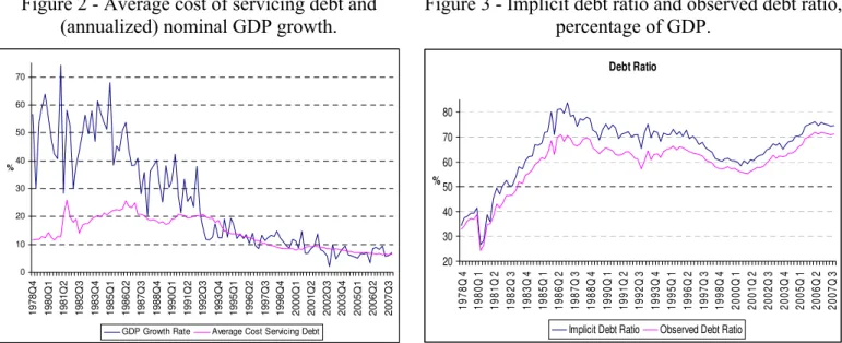
Figure 2 plots the average debt cost servicing and the nominal (annualized) GDP

growth. It shows that Portugal, in general, has moved from a situation where nominal

GDP growth exceeded the cost of financing the debt to a situation where the converse

has been true.

In addition, Figure 3 displays the observed debt-to-GDP ratio and the implicit

debt-to-GDP ratio, that is, the one that emerges from the government debt’s feedback.

As can be seen, the implicit series for the debt-to-GDP ratio tracks pretty well the actual

series.14

[Figure 2]

[Figure 3]

Finally, the quarterly series of government spending and revenues are computed

using the monthly Central Government’s cash data. Figure 4 provides a comparison of

the annual values of such data with the annual national accounts data provided by the

13 The average government debt cost is obtained by dividing the net interest payments by the government debt at time t−1.

(14)

European Commission (Ameco database). The patterns of both series are rather

similar.15

[Figure 4]

5.2 Results

The starting point is the estimation of a B-SVAR model that does not include the

feedback from government debt, that is, where equation (2) is not considered. Then, we

compare the results with the ones that emerge from estimating specifications (1), (2),

and (3).

Figure 5 shows the impulse-response functions to a fiscal policy shock. The

solid line refers to the median response when the VAR is estimated without the

government budget constraint, and the dashed lines are, respectively, the median

response and the 68 percent posterior confidence intervals from the VAR estimated by

imposing the government budget constraint. The confidence bands are constructed using

a Monte Carlo Markov-Chain (MCMC) algorithm based on 1000 draws.

[Figure 5]

Figure 5a displays the impulse-response functions of all variables in Xt to a

positive shock in government spending. In the case we do not include the debt feedback,

it can be seen that government spending declines steadily following the shock, and the

effect roughly vanishes after four quarters. The effects on GDP are negative and reveal

that government spending has a strong “crowding-out” effect on the private sector. In

fact, both private consumption and private investment fall after the shock. These results

are in line with the works of Giavazzi and Pagano (1990) and Alesina and Ardagna

(1998) who uncovered the presence of “non-Keynesian effects” (i.e., negative spending

multipliers) during large fiscal consolidations.

In addition, there is a positive effect on the average cost of debt that reaches its

peak after six quarters. The price level is also impacted persistently and positively by

the shock in government spending. Finally, the results suggest that after a government

spending shock, there is an increase in government revenue which is, however, small.

(15)

Therefore, this suggests that an expansion of government spending is associated with a

episode of fiscal deterioration.

When we include the debt dynamics in the model, the effects of a government

spending shock on the average cost of debt become somewhat larger while the impact

on GDP is marginally smaller. Additionally, investment falls much more than before

and the positive impact on the price level is attenuated by the feedback from

government debt.

Figure 5b shows the impulse-response functions to a positive shock in

government revenue. The results suggest that government revenue declines steadily

following the shock which erodes after two quarters. The effects on GDP, private

consumption and private investment are slightly positive over the four quarters

following the shock, but they quickly mean revert and become negative.16 In contrast,

the price level falls for about four quarters, then recovers, and becomes positive. These

results are closely related to the reaction of government spending, which increases after

the shock. In fact, an increase in government revenue is followed by a somewhat less

disciplined fiscal policy and, as a result, there is a deterioration of the fiscal balance.

This also seems to be the reason for the positive impact on the average cost of debt.

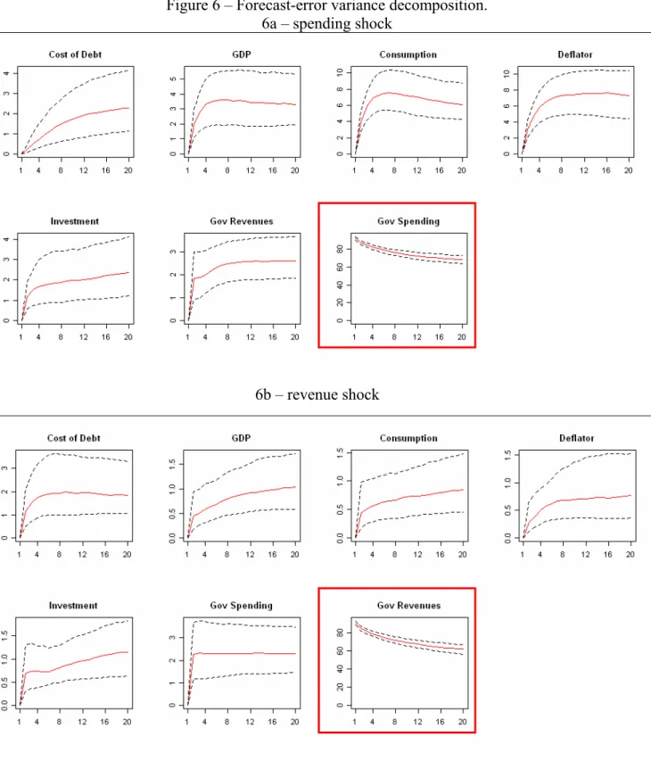
Figure 6 shows the forecast-error variance decompositions to a fiscal policy

shock when we include the feedback from government debt. The solid line corresponds

to the median estimate, and the dashed lines indicate the 68 percent posterior confidence

intervals estimated by using a MCMC algorithm based on 1000 draws.

[Figure 6]

Figure 6a plots the forecast error-variance decomposition of all variables in Xt to

a shock in government spending. It shows that government spending shocks explain a

large percentage (around 80%) of their own forecast-error variance decomposition. It

also accounts for between 6% and 8% of the forecast-error variance decomposition of

private consumption and the price level, and a small share of the remaining variables.

(16)

Figure 6b summarizes the forecast error-variance decomposition of the variables

in the system to a shock in government revenue. Similarly to the case of government

spending, government revenue shocks account for a large fraction of their own

forecast-error variance decomposition. On the other hand, government revenue shocks play a

negligible role for all the remaining variables.

5.3 Fiscal shocks and government debt feedback

In this sub-section, we consider the potential debt feedback and estimate the

following structural VAR:

t t

i t

t X d d c

X +Γ + +γ − = +ε

Γ₀ ₁ ₋₁ ... ( ₋₁ *) , (7)

1

(1 )(1 )

t t t

t t

t t t t

i G T

d d

PY

π µ −

+ −

= +

+ + . (8)

Specification (7) is suggested by Bohn (1998) who estimates a fiscal reaction

function in which d* is the unconditional mean of the debt ratio. Therefore, we model

the target level of the debt as a constant on the basis of the evidence of stationarity of d.

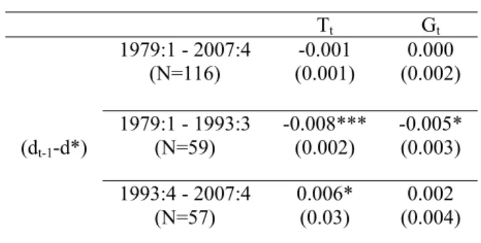
Table 1 reports the estimated coefficients on (dt−1 − d*) in the structural

equations of the SVAR (government spending and government revenue). We report the

coefficients (and the standard errors in brackets) taken from the estimation for the full

sample and for sub-samples. We consider two sub-samples: 1979:1 – 1993:3,

corresponding to the period before the Maastricht Treaty entered into force; and 1993:4

– 2007:4, thereafter.

Table 1 – The effect of (dt-1-d*) in a VAR.

Tt Gt

1979:1 - 2007:4 (N=116)

-0.001 (0.001)

0.000 (0.002)

(dt-1-d*)

1979:1 - 1993:3 (N=59)

-0.008*** (0.002)

-0.005* (0.003)

1993:4 - 2007:4 (N=57)

0.006* (0.03)

0.002 (0.004)

Note: standard errors in brackets.

*, **, *** - statistically significant respectively at the 10%, 5%, and 1% levels.

In general, the results do not show a significant response of revenue and primary

spending to deviations of the debt-to-GDP ratio from its sample average for the full

(17)

weak stabilizing effect that works mainly through government spending: when the

debt-to-GDP ratio is above its historical mean, government primary spending decreases (the

coefficient associated to (dt−1 − d*) is negative (-0.005). In the second sub-sample

(1993:4 – 2007:4), the empirical findings show that government revenue plays some

stabilizing effect: when the debt-to-GDP ratio is above its historical mean, government

revenue increases as the coefficient associated to (dt−1− d*) is positive (0.006).

5.4 A VAR counter-factual exercise

We now conduct a VAR counter-factual exercise aimed at describing the effects

of shutting down the shocks in government spending or government revenue. In

practice, after estimating the VAR summarized by (1), (2) and (3), we construct the

counter-factual (CFT) series as follows:

{ CFT t t i CFT t CFT t t i n CFT t n n c d X X d X

L +γ =Γ +Γ + +γ = +ε

Γ ₋ ₋ ₋

× × 1 1 1 0 1 1 ... )

( ₁₂₃ ₍₉₎

1

(1 )(1 )

t t t

t t

t t t t

i G T

d d

PY

π µ −

+ −

= +

+ + (10)

CFT t 1 0 ε − Γ = CFT t

v . ₍₁₁₎

This is equivalent to consider the following vector of structural shocks

'

0, , , , , ,

CFT T Y P i I C t t t t t t t

ε _{= ⎣}⎡ ε ε ε ε ε ε ⎤_⎦ ₍₁₂₎

'

, 0, , , , ,

CFT G Y P i I C t t t t t t t

ε _{= ⎣}⎡ε ε ε ε ε ε ⎤_⎦ _(13),

where we shut down, respectively in (12) and in (13), the government spending and the

government revenue unexpected variation and then use the counter-factual structural

shocks to build the counter-factual series for all endogenous variables of the system.

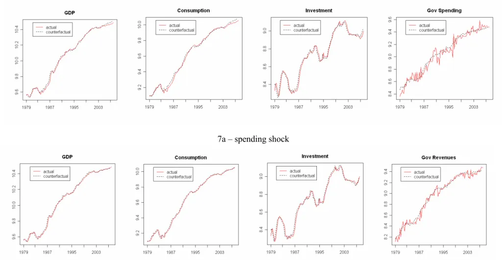
Figure 7a plots the actual and the counter-factual series for GDP, private

consumption, private investment, and government spending in the case of a shock to

government spending. Figure 7b displays the actual and the counter-factual series for

GDP, private consumption, private investment, and government revenue in the case of a

shock to government revenue.

[Figure 7]

The results show that fiscal policy shocks play a minor role as the difference

(18)

can see that in the absence of government spending shocks, private consumption and

private investment would have been higher, for instance, in the period 1983-1988 and,

more recently, since 2003. Therefore, such evidence suggests and confirms that

unexpected increases in government spending generate relevant “crowding-out” effects.

In the case of government revenue, the difference between the actual and the

counterfactual series are negligible, a feature that may be related with the relative size

of the government revenue shocks. In fact, while unexpected variation in government

spending seems to be large – as one can see by looking at the larger differences between

the actual government spending and the counter-factual government spending -,

government revenue shocks are generally small.

6. Conclusion

This paper evaluates the macroeconomic effects of fiscal policy in Portugal for

the period 1979:1-2007:4, drawing on a new set of quarterly data built from the monthly

Central Government’s cash data.

We identify fiscal policy shocks using a recursive partial scheme, and estimate a

Bayesian Structural Vector Autoregression, therefore, accounting for the posterior

uncertainty of the impulse-response functions.

The empirical evidence suggests that government spending shocks: (i) have, in

general, a negative effect on GDP; (ii) lead to a fall of both private consumption and

private investment; and (iv) impact persistently and positively on the price level and the

average cost of refinancing the debt. In addition, government revenue shocks: (i) have a

negative impact on GDP, on private consumption and on private investment, although

the response emerges with a lag of about four quarters; and (ii) lead to a fall in the price

level.

These results suggest that an expansion of government spending is associated to

an episode of fiscal deterioration. Similarly, an increase in government revenue is

followed by a somewhat less disciplined fiscal policy.

When we explicitly consider the feedback from government debt, (long-term)

interest rates and GDP become more responsive and the effects of fiscal policy on these

variables also become more persistent. In addition, the results provide weak evidence of

stabilizing effects of the debt level on the primary budget balance.

Finally, a VAR counter-factual exercise shows that unexpected spending shocks

(19)

References

Afonso, A. (2008a), “Ricardian Fiscal Regimes in the European Union”, Empirica,

35(3), 313–334.

Afonso, A. (2008b), “Expansionary fiscal consolidations in Europe: new evidence”,

Applied Economics Letters, DOI http://dx.doi.org/10.1080/13504850701719892,

forthcoming.

Afonso, A. (2007). “Public finances in Portugal: a brief long-run view”, Department of

Economics, ISEG-UTL, Working Paper Nº. 1/2007/DE/CISEP/UECE.

Afonso, A. (2005). “Fiscal Sustainability: the Unpleasant European Case,”

FinanzArchiv, 61(1), 19-44.

Afonso, A.; Claeys, P. (2008), “The dynamic behaviour of budget components and

output”, Economic Modelling, 25, 93-117.

Afonso, A., and Fernandes, S. (2008). “Assessing hospital efficiency: non-parametric

evidence for Portugal”, Department of Economics, ISEG-UTL, Working Paper Nº.

07/2008/DE/UECE.

Afonso, A., and Sousa, R. M. (2009a), “The macroeconomic effects of fiscal policy”,

ECB Working Paper Nº. 991.

Afonso, A., and Sousa, R. M. (2009b), “Fiscal policy, housing and stock prices”, ECB

Working Paper Nº. 990.

Alesina A.; Ardagna, S. (1998), “Tales of fiscal adjustment”, Economic Policy, 27,

489-545.

Barro, R. J. (1974), "Are government bonds net wealth?", Journal of Political Economy,

82(6), 1095-1117.

Bauwens, L.; Lubrano, M.; Richard, J.-F. (1999), Bayesian inference in dynamic

econometric models, Oxford University Press, Oxford.

Beetsma, R.; Jensen, H. (2005), “Monetary and fiscal policy interactions in a

Micro-Founded Model of a Monetary Union”, Journal of International Economics, 67,

320-352.

Biau, O.; Girard, E. (2005), “Politique budgétaire et dynamique économique en France:

l'approche VAR structurel.”, Économie et Prévision, 169–171, 1–24.

Blanchard, O. (2007). “Adjustment within the Euro: The Difficult Case of Portugal”,

(20)

Blanchard, O.; Perotti, R. (2002), "An empirical characterization of the dynamic effects

of changes in government spending and taxes on output", Quarterly Journal of

Economics, 117(4), 1329-1368.

Bohn, H. (1998), "The Behaviour of U.S. public debt and deficits", Quarterly Journal of

Economics, 113, 949-963.

Canzoneri, M.; Cumby, R.; Diba, B. (2001), "Is the price level determined by the needs

of fiscal solvency”, American Economic Review, 91(5), 1221-1238.

Chung, H.; Davig, T.; Leeper, E. M. (2007), “Monetary and fiscal switching”, Journal

of Money, Credit and Banking, 39(4), 809-842.

Constâncio, V. (2005). “European monetary integration and the Portuguese case” in

Detken, C.; Gaspar, V. and Noblet, G. (eds.), The new European Union Member

States: convergence and stability, ECB.

De Castro Fernández, F.; Hernández De Cos, P. (2006), “The economic effects of

exogenous fiscal shocks in Spain: a SVAR approach”, ECB Working Paper Nº. 647.

Edelberg, W.; Eichenbaum, M.; Fisher, J. (1999), “Understanding the effects of a shock

to government purchases”, Review of Economics Dynamics, 2, 166–206.

Fatás, A.; Mihov, I. (2001), “The effects of fiscal policy on consumption and

employment: theory and evidence”, CEPR Discussion Paper Nº. 2760.

Favero, C.; Giavazzi, F. (2007), "Debt and the effects of fiscal policy", University of

Bocconi, Working Paper Nº. 317.

Giavazzi, F.; Pagano, M. (1990), “Can severe fiscal contractions be expansionary? Tales

of two small european countries”, in Blanchard, O. J.; Fischer, S. (eds.), NBER

Macroeconomics Annual, MIT Press, 75–110.

Giavazzi, F.; Jappelli, T.; Pagano, M. (2000), "Searching for non-linear effects of fiscal

policy: evidence from industrial and developing countries", European Economic

Review, 44(7), 1259-1289.

Giordano, R.; Momigliano, S.; Neri, S.; Perotti, R. (2007), “The effects of fiscal policy

in Italy: Evidence from a VAR model”, European Journal of Political Economy, 23,

707-733.

Guichard, S. and Leibfritz, W. (2006). “The Fiscal Challenge in Portugal”, OECD

Heppke-Falk, K.H.; Tenhofen, J.; Wolff, G. B. (2006), “The macroeconomic effects of

exogenous fiscal policy shocks in Germany: a disaggregated SVAR analysis”,

(21)

Kormendi, R. C. (1983), “Government debt, government spending, and private sector

behavior”, American Economic Review, 73, 994-1010.

Marinheiro, C. (2006). “Sustainability of Portuguese Fiscal Policy in Historical

Perspective”, Empirica, 33(2-3), 155-179.

Mountford, A.; Uhlig, H. (2005), "What are the effects of fiscal policy shocks?",

Humboldt-Universität zu Berlin Working Paper SFB Nº. 649.

Pérez, J. (2007). “Leading indicators for euro area government deficits”, International

Journal of Forecasting, 23, 259-275.

Onorante, L; Pedregal, D.; Pérez, J. and Signorini, S. (2008). “The usefulness of

infra-annual government cash budgetary data for fiscal forecasting in the euro area,” ECB

Perotti, R. (1999), “Fiscal policy in good times and bad”, Quarterly Journal of

Economics, 114, 1399-1436.

Perotti, R. (2004), "Estimating the effects of fiscal policy in OECD countries",

University of Bocconi, Working Paper.

Pina, A. (2004). “Fiscal Policy in Portugal: Discipline, Cyclicality and the Scope for

Expenditure Rules”, proceedings of the 2nd Conference on Portuguese Economic

Development in the European Context, held by the Bank of Portugal in Lisbon,

11-12 March 2004, 15-65.

Ramey, V.; Shapiro, M. (1998), “Costly capital reallocation and the effects of

government spending”, Carnegie Rochester Conference on Public Policy, 48,

145-194.

Romer, C.; Romer, D. H. (2007), "The macroeconomic effects of tax changes: estimates

based on a new measure of fiscal shocks", NBER Working Paper Nº. 13264.

Schervish, M. J. (1995), Theory of statistics, Springer, New York.

Zellner, A. (1971). An introduction to bayesian inference in econometrics, Wiley, New

(22)

Appendix A. Confidence bands of the impulse-response functions

Under the normalization of Λ =I _{, the impulse-response function to a one}

standard-deviation shock is given by:

. ) (L −1Γ₀−1

B _(A.1)

We assess uncertainty regarding the impulse-response functions by following

Sims and Zha (1999). Therefore, we construct confidence bands by drawing from the

Normal-Inverse-Wishart posterior distribution of B(L) and Σ

) ) ' ( , ( ~

| 1

^

− Σ Ν β Σ⊗ X X

β (A.2)

) , ) (( Wishart

~ ^ 1

1 _TΣ _T −_m

Σ− −

(A.3)

where β is the vector of regression coefficients in the VAR system, Σ is the covariance

matrix of the residuals, the variables with a hat denote the corresponding

maximum-likelihood estimates, X is the matrix of regressors, T is the sample size and m is the

number of estimated parameters per equation (see Zellner, 1971; Schervish, 1995; and

Bauwens et al., 1999).

Appendix B. Data description and sources

GDP

Data for GDP are quarterly, seasonally adjusted, and comprise the period 1978:1-2007:4. The source is the Bank of Portugal.

Private Consumption

The source is the Bank of Portugal. Consumption is defined as the household consumption expenditure including non-profitable institutions serving households. Data are quarterly, seasonally adjusted, and comprise the period 1978:1-2007:4.

Price Deflator

All variables were deflated by the GDP deflator (2000=100). Data are quarterly, seasonally adjusted, and comprise the period 1978:1-2007:4. The source is the Bank of Portugal.

Private Investment

The source is the Bank of Portugal. Private Investment is defined as total gross fixed capital formation. Data are quarterly, seasonally adjusted, and comprise the period 1978:1-2007:4.

Government Spending

(23)

authorized expenditure and debt interest payments. We seasonally adjust quarterly data using Census X12 ARIMA, and the series comprise the period 1978:1-2007:4.

Interest Payments

The source is the Bank of Portugal, collected from the Monthly Bulletin of the Directorate-General of Public Accounting. Interest Payments is defined as Central Government debt interest payments (on a cash basis). We seasonally adjust quarterly data using Census X12 ARIMA, and the series comprise the period 1978:1-2007:4.

Government Revenue

The source is the Bank of Portugal, collected from the Monthly Bulletin of the Directorate-General of Public Accounting. Government Revenue is defined as Central Government total revenue (on a cash basis). We seasonally adjust quarterly data using Census X12 ARIMA, and the series comprise the period 1978:1-2007:4.

Government Debt

The source is the Bank of Portugal, the Directorate-General of Treasury, and the Directorate-General of Public Credit. Government Debt is defined as the stock of Direct State Debt.

The original series are available as follows: 1.

a) Total Internal Debt, for the period 1997:12-1994:6, on a quarterly basis; b) Internal Direct Debt, for the period 1997:12-1994:6, on a quarterly basis; c) Total External Debt, for the period 1997:12-1994:6, on a quarterly basis; d) Direct External Debt, for the period 1997:12-1994:6, on a quarterly basis; e) Total Public Debt, for the period 1997:12-1994:6, on a quarterly basis; f) Effective Public Debt, for the period 1997:12-1994:6, on a quarterly basis; 2.

a) Internal Effective Direct Debt, for the periods 1991:12, 1992:12, and 1993:6-1995:11, on a monthly basis;

b) Total Effective Direct Debt, for the periods 1991:12, 1992:12, and 1993:6-1995:11, on a monthly basis

3.

a) Internal Direct Debt, for the period 1995:7-1998:12, on a monthly basis; b) Total Direct Debt, for the period 1995:7-1998:12, on a monthly basis 4.

a) Direct State Debt, for the period 1998:12-2007:4, on a monthly basis.

We build the series for the Direct State Debt as follows:

1) For the period 1998:12-2008:4, as the series of Direct State Debt itself;

2) For the period 1995:7-1997:12, we use the ratio of Direct State Debt to Total State Debt in 1998:12 (that is, a scale factor of 0.994679113), to back-out the series of Direct State Debt;

3) For the period 1993:6-1995:6, we use the ratio of Total Effective Direct State Debt to Total Direct State Debt in the period 1995:7-1995:11 (that is, a scale factor of 1.002277388), to back-out the series of Total Direct Debt;

(24)

Given that the scale factors are very close to one, the time series of the Direct State Debt is smooth over time and we guarantee that there are not structural breaks.

We build the quarterly series using monthly data (where available) and seasonally adjust it using Census X12 ARIMA. The constructed series comprise the period 1977:4-2007:4.

Average Cost of Financing Debt

The average cost of financing debt is obtained by dividing interest payments by debt at time t-1.

Long-Term Interest Rate

(25)

Figure 1 – Monetary conditions and fiscal balances in Portugal (2000-2008).

Change in cyclically adjusted primary balance

2001 2005 2000 2004 2007 2002 2006 2008 2003 -3.5 -3.0 -2.5 -2.0 -1.5 -1.0 -0.5 0.0 0.5 1.0 1.5 2.0

-3.0 -2.0 -1.0 0.0 1.0 2.0 3.0

C h a nge in r e a l s hor t-te rm int e re s t r a te ( E u ribo r 6 m

) _{Fiscal easing,}

Monetary tightening Fiscal easing, Monetary easing Fiscal tightening, Monetary tightening Fiscal tightening, Monetary easing EDP

Source: EC, Eurostat, Banco de Portugal, and own calculations.

Notes: HICP, September 2008, Euribor, October 2008, and EC Autumn 2008 forecasts for CAPB in 2008. EDP – Excessive Deficit Procedure.

Figure 2 - Average cost of servicing debt and (annualized) nominal GDP growth.

Figure 3 - Implicit debt ratio and observed debt ratio, percentage of GDP.

0 10 20 30 40 50 60 70 1978Q 4 1980Q 1 1981Q 2 1982Q 3 1983Q 4 1985Q 1 1986Q 2 1987Q 3 1988Q 4 1990Q 1 1991Q 2 1992Q 3 1993Q 4 1995Q 1 1996Q 2 1997Q 3 1998Q 4 2000Q 1 2001Q 2 2002Q 3 2003Q 4 2005Q 1 2006Q 2 2007Q 3 %

GDP Growth Rate Average Cost Servicing Debt

Debt Ratio 20 30 40 50 60 70 80 1978Q 4 1980Q 1 1981Q 2 1982Q 3 1983Q 4 1985Q 1 1986Q 2 1987Q 3 1988Q 4 1990Q 1 1991Q 2 1992Q 3 1993Q 4 1995Q 1 1996Q 2 1997Q 3 1998Q 4 2000Q 1 2001Q 2 2002Q 3 2003Q 4 2005Q 1 2006Q 2 2007Q 3 %

Implicit Debt Ratio Observed Debt Ratio

(26)

Figure 4 – Quarterly versus annual fiscal data.

Primary Spending

25 35 45 55

1978 1983 1988 1993 1998 2003

% GDP

from quarterly data AMECO

Total Spending

0 10 20 30 40 50 60

1978 1983 1988 1993 1998 2003

% GDP