The use of genetic programming for detecting the incorrect predictions of classification models

(1)

The use of Genetic Programming for detecting

the incorrect predictions of Classification Models

Adrianna Maria Napiórkowska

Dissertation presented as partial requirement for obtaining

the Master’s degree in Advanced Analytics

(2)

Title: The use of Genetic Programming for detecting the incorrect

predictions of Classification Models Adrianna Maria Napiórkowska

MAA

20

(3)

(4)

NOVA Information Management School

Instituto Superior de Estat´ıstica e Gest˜ao de Informa¸c˜ao

Universidade Nova de Lisboa

The use of Genetic Programming for detecting the

incorrect predictions of Classification Models

by

Adrianna Maria Napi´orkowska

Dissertation presented as partial requirement for obtaining the Master’s degree in Advanced Analytics

Advisor: Leonardo Vanneschi

(5)

Abstract

Companies around the world use Advanced Analytics to support their decision making process. Traditionally they used Statistics and Business Intelligence for that, but as the technology is advancing, the more complex models are gaining popularity. The main reason for an increasing interest in Machine Learning and Deep Learning models is the fact that they reach a high predic-tion accuracy. On the second hand with good performance, comes an increasing complexity of the programs. Therefore the new area of Predictors was intro-duced, it is called Explainable AI. The idea is to create models that can be understood by business users or models to explain other predictions. Therefore we propose the study in which we create a separate model, that will serve as a veryfier for the machine learning models predictions. This work falls into area of Post-processing of models outputs. For this purpose we select Genetic Programming, that was proven to be successful in various applications. In the scope of this research we investigate if GP can evaluate the prediction of other models. This area of applications was not explored yet, therefore in the study we explore the possibility of evolving an individual for another model validation. We focus on classification problems and select 4 machine learn-ing models: logistic regression, decision tree, random forest, perceptron and 3 different datasets. This set up is used for assuring that during the research we conclude that the presented idea is universal for different problems. The performance of 12 Genetic Programming experiments indicates that in some cases it is possible to create a successful model for errors prediction. During the study we discovered that the performance of GP programs is mostly connected to the dataset on the experiment is conducted. The type of predictive models does not influence the performance of GP. Although we managed to create good classifiers of errors, during the evolution process we faced the problem of overfitting. That is common in problems with imbalanced datasets. The results of the study confirms that GP can be used for the new type of problems and successfully predict errors of Machine Learning Models.

Keywords: Machine Learning, Explainable AI, Post-processing, Classification, Genetic Programming, Errors Prediction

(6)

(7)

List of Figures

2.1 Types of machine learning problems . . . 14

2.2 Machine learning process . . . 15

2.3 Deep Learning solution . . . 15

2.4 Modified machine learning process . . . 16

3.1 Example of a tree generation process using full method . . . 23

3.2 Example of a tree generation process using grow method . . . . 24

3.3 Example of subtree crossover . . . 26

3.4 Example of subtree mutation . . . 27

4.1 Visualization of the test cases preparation . . . 32

4.2 Datasets transformations used in experimental study and steps applied in the process. . . 33

4.3 Distribution of dependent variable in Breast Cancer Wisconsin dataset . . . 36

4.4 Distribution of dependent variable in Bank Marketing dataset . 37 4.5 Distribution of target variable in Polish Companies Bankruptcy dataset before and after up-sampling . . . 38

4.6 Implementation of the research idea . . . 41

4.7 Data split conducted in the project . . . 41

4.8 Summary of the results for: Breast Cancer Wisconsin Dataset Test Cases . . . 47

4.9 Summary of the results for: Bank Marketing Dataset Test Cases 50 4.10 Summary of the results for: Polish Companies Bankruptcy Dataset Test Cases . . . 52

4.11 Comparison of the performance of the best GP programs from different runs calculated on the test set . . . 54

4.12 Average of Maximum Train Fitness summarized by Model and Test Case . . . 55

(10)

(11)

List of Tables

4.1 Summary of the predictions used as test cases . . . 39

4.2 Comparison between Confusion Matrices obtained by 2 different

Fitness Functions . . . 44

4.3 Summary of the parameters selected for test cases . . . 45

4.4 Best Individuals found for Breast Cancer Wisconsin Dataset

Test Cases . . . 48

4.5 Best Individuals found for Bank Marketing Dataset Test Cases . 51

4.6 Best Individuals found for Polish Companies Bankruptcy Dataset

(12)

(13)

Chapter 1 Introduction

The history of algorithms begins in 18th century, when Ada Lovelace, a math-ematician and poet, have written an article describing a concept that would allow the engine to repeat a series of instructions. This method is known nowadays as loops, widely known in computer programming. In her work, she describes how code could be written for a machine to handle not only numbers, but also letters and commands. She is considered the author of first algorithm and first computer programmer.

Although Ada Lovelace did not have a computer as we have today, the ideas she developed are present in various algorithms and methods used nowadays. Since that time, the researches and scientist were focused on optimization of work and automation of repetitive tasks. Over the years they have developed a wide range of methods for that purpose. In addition to that the objective of many researches was to allow computer programs to learn. This ability could help in various areas, starting from learning how to treat diseases based on medical records, apply predictive models in areas where classic approaches are not effective or even create a personal assistant that can learn and optimize our daily tasks. All of the mentioned concepts can be described as machine learning.

According to Mitchell (1997), an understanding of how to make computers learn would create new areas for customization and development. In addition, the detailed knowledge of machine learning algorithms and the ways they work, might lead to a better comprehension of a human learning abilities. Many com-puter programs were developed by implementing useful types of learning and they started to be used in commercial projects. According to research, these algorithms were outperforming other methods in the various areas, like speech or image recognition, knowledge discovery im large databases or creating a program that would be able to act like human e.g chat bots and game playing programs.

(14)

CHAPTER 1. INTRODUCTION

On the one hand intelligent systems are very accurate and have high pre-dictive power. They are also described by a large number of parameters, hence it is more difficult to draw direct conclusions from the models and trust their predictions. Therefore the research in an area of explainable AI started to be very popular and there was a need for analysis of the output of predictive mod-els. There are areas of study or business applications that especially require transparency of applied models, e.g. Banking and the process of loans ap-proval. One reason for that are new regulations protecting personal data - like General Data Protection Regulation (GDPR), which require entrepreneurs to be able to delete sensitive personal data upon request and protect consumers with new right - Right of Explanation. It is affecting business in Europe since May 2018 and is causing an increasing importance ofthe field of Explainable AI as mentioned in publication: Current Advances, Trends and Challenges of Machine Learning and Knowledge Extraction: From Machine Learning to Ex-plainable AI by Holzinger et al. (2018). The applications of AI in many fields is very successful, but as stated in mentioned article:

We are reaching a new AI spring. However, as fantastic current approaches seem to be, there are still huge problems to be solved: the best performing models lack transparency, hence are considered to be black boxes. The general and worldwide trends in privacy, data protection, safety and security make such black box solutions difficult to use in practice.

Therefore in order to align with this regulation and provide trust-worthy predictions in many cases the additional step of post-processing of the predic-tions is applied. A good model should generate decisions with high certainty. First of the indication for that is high performance observed during training phase. Secondly the results of evaluation on the test and validation sets should not diverse significantly, proving stability of the solution. In this area, the use of post-processing of outputs can be very beneficial. It the model is predicting loans that will not be repaid, then the cost of wrong prediction can be very high, if the loan will be given to the bad consumer. Therefore banking insti-tution spend a lot of time and resources on improving their decision making process.

Another common technique is using for making a prediction a model that is more transparent than other and can be easily understood by the business stakeholders and explained to the client. The example of a black boxes are artificial neural networks, mainly to the fact that they have large number of parameters to tune and if the architecture of such model is complex, the original inputs: variables are transformed to such stage, that the conclusions cannot be drawn from them. The answer to that issue can be a model that is transparent, e.g. Decision Tree.

(15)

CHAPTER 1. INTRODUCTION

The objective of this research is to check if one model can be used for the evaluation of the predictions generated by other machine learning models. This means that we want to combine 2 aspect of an analysis: the prediction of errors, for single-prediction evaluation and use white box model for better understanding of the generated models. For the purpose of this study we picked Genetic Programming as a method for evaluation. It is a method that is proven to be successful in various problems and business areas, but also is considered to be explainable as stated by Howard and Edwards (2018) during International Conference on Machine Learning and Data Engineering (iCMLDE) in 2018. The authors ot the paper presented a project in which they were able to provide an equivalent GP model to an existing black box model. In order to test this approach we select few data sets and different models to make a study comprehensive.

The expected results of this research is to obtain a model that will predict the errors of machine learning models correctly and will be explainable. If the stated objectives will be met, the resulting individuals would prove that the post-processing of predictions is possible. Furthermore we may conclude that the evolved individuals can be used in various fields for minimizing the risk of bad decisions. They could be applied in any business problem in which the cost of incorrect prediction is high. As the examples of the business areas with high cost of incorrect predictions are banking or healthcare. The companies from these fields focus on Explainable Models that produces trust-worthy pre-dictions to avoid giving loans to bad clients or to correctly assign treatment to the particular disease.

In this thesis we present the outcome of the study and we structure the text as follows. In the first chapter we introduce the problem of understanding a machine learning models and their applications. We focus on the process of developing such a model and how to include additional evaluation step in it. Furthermore we discuss the known solutions for additional verification of the predictions and deep learning models explanation. In the next chapter we present Genetic Programming - a method that was selected for this project in order to check if they can be used as a veryfier. In this chapter we present the basic structure of a project that uses genetic programming. We describe the basic methods used in an evolution process as well as applications of GP. In chapter 3, we present the design of the study, that we conducted. We present models used for generating predictions and the way of evaluating the results. Chapter 4 contains the description of all test cases that we used in the research, with description of the data sets, experimental setting and the summary of the results. Finally, in chapter 5 we summarize the project and set the objectives for possible future work.

(16)

(17)

Chapter 2 Machine Learning

For the last two centuries algorithms and computer programming became a key element in every company. They are used for optimization of the processes, cutting costs and increasing revenues. The solutions based on data analytics cover different areas in an organization. Starting from the simple descriptive statistics for day-to-day monitoring of a business condition, through algorithms used for optimization of complex tasks that require analysis of big volume of data, to artificial intelligence systems that can predict events crucial for busi-ness and detect hidden patterns in the data. The last type of applications can be described as advanced analytics and an important part of it is Machine Learning (ML) - the group of algorithms that by means of an iterative process learn from data.

The computer program that learns can be defined as:

A computer program is said to learn from experience E with re-spect to some class of task T and performance measure P , if its performance at tasks in T , as measured by P , improves with E.

Tom M Mitchell, 1997 Machine learning is a combination of mathematics, algorithms and statis-tics that allows to create computer programs that are able to perform spe-cific task without providing direct instructions. As described in the book by Mitchell (1997), they analyze the training data observation by observation, gaining experience, in order to perform defined task. Previously the data were analyzed by the employees. They used to analyze data and discover various patterns, then they would transform their findings into rules. Now, with assis-tance of an artificial intelligence, algorithms are able to gain knowledge from data by gradually improving their performance. This process is called learning.

(18)

CHAPTER 2. MACHINE LEARNING

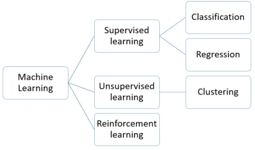
Within all set of machine learning tasks, there are 3 main types: supervised learning, unsupervised learning and reinforcement learning. Within the first group of problems, the task is to fit a model based on set of labeled data in a training set, that will be giving good predictions on the test set. The labels can be either discrete categories or continues values, by this distinction we can further group the tasks into classification and regression. The second group of problems is unsupervised learning. The goal there is to understand underlying pattern in the dataset or group observations into clusters with similar charac-teristics. The last type of tasks is reinforcement learning. These problems are different from the previous groups as there is no dataset or training data. The objective is to train an agent that will be performing a defined task. It can be done by repetitively exposing it to a task and grant a reward for good action and punishment for wrong action.

Figure 2.1: Types of machine learning problems

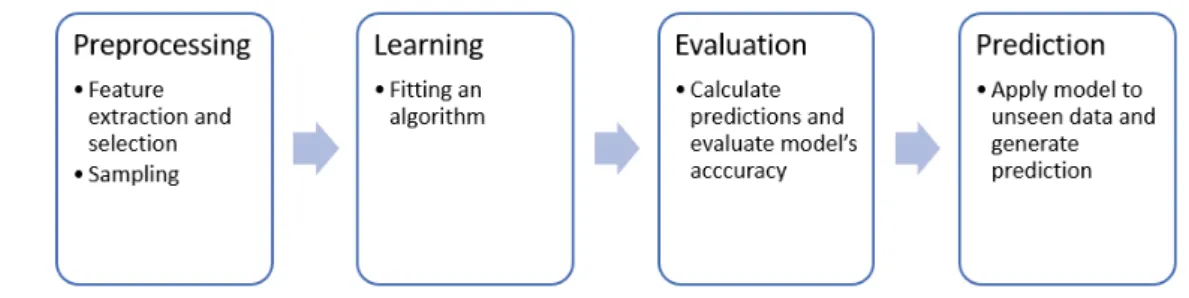
The process of creating a machine learning model for a supervised learning problem can be described in 4 steps, according to the diagram presented on the Figure 2.2. In order to start fitting process, needed pre-processing must be done. In this stage of the project an analyst reviews the dataset in order to remove or impute missing values, extract good features or remove bad ones and sample the dataset if some group of observations is not well represented in the dataset. Then after preparing a dataset, the learning process can start. In this step, various algorithms are used to fit a good model that performs a defined task. It is done by optimizing parameters in the algorithms and feeding

(19)

them with data. The optimization process is done by evaluating a model on the unseen data. If the accuracy of the model is not satisfactory there is a need for additional training or adjustment of the parameters. And if the evaluated program fulfill the requirements, it can be applied for the new set of data and work as a classifier.

Figure 2.2: Machine learning process

2.1 Models interpretability

Machine learning and artificial intelligence are becoming more and more com-plex. There are few reasons for that. Firstly, there are databases and systems that allow collecting big volumes of data. In addition to that, there are com-puters that allow much faster computations, making development of complex models possible. Unfortunately there is a trade-off between high accuracy and simplicity. In order to create a classifier that is able to recognize various items on an image or predict some unusual event, we need to reach for models with large number of inputs and parameters, hence they are no longer understand-able for a human.

(20)

In some of the areas, when models are used for boosting click rates for advertisements or tagging images in the online store, we do not need additional

analysis for the predictions. If these models are helping to automate and

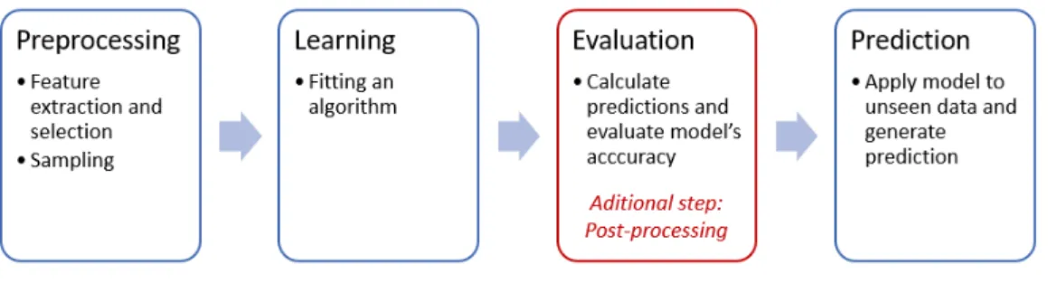
optimize repeatable processes and their accuracy is high, it is enough. On the other hand there are areas, where either due to governmental regulations or due to the need for prevent unfair decisions, there is a need to document the reasons for a particular prediction and understand the choice a classifier. In these cases to the standard machine learning process we need to add additional step in an evaluation phase, which is post-processing. The reason for doing that is building a trust in the model, which is very important if someone is going to make decisions based on it. The diagram for the modified machine learning process is presented on the figure 2.4.

Figure 2.4: Modified machine learning process

The interpretability of applied solution can be beneficial in many ways. Firstly we can understand which features or parts of an image are responsible for a prediction, hence we can have more trust in a model. It can also serve as an additional checking point for machine learning systems to avoid overfitted or too complex models. An analysis of the outputs combined with the classic exploratory data analysis can lead to understand patterns in the training set that could lead into better understanding of a specific topic. It may also lead to creation of new features that can improve final accuracy. Furthermore, the post-processing of the predictions can help to investigate the errors, focusing on the specific variables that are causing them or particular observations that are harder to predict.

The objective of the research summarized in this work is to check if spe-cific kind of Artificial Intelligence models - Genetic Programming could be beneficial for predicting the errors in machine learning models predictions. In addition the aspect of the error cases analysis by means of GP evolution will be discussed.

(21)

2.2 Explainable AI

Advanced data analysis is present in almost every industry and many areas of our lives. In many areas in addition to creation of good classifier, there is a need to make this model explainable. Therefore the research on post-processing of machine learning models and their predictions became very popular. In the previous section we provided different advantages of including post-processing in the machine learning project in order to make it more understandable for humans. In this section we discuss available methods for investigation of ma-chine learning models and its predictions.

As Ribeiro et al. (2016) explains in his article Why should I trust you?, while companies are using machine learning models as tools or they are integrating them within other products, their main concern is the trust in a model. If the users do not trust a model or its prediction, they are not going to use it and its development is not beneficial. Additionally he highlights the two types of trust, when it comes to the model itself and each prediction it generates. Firstly, we want to make sure that model will behave reasonably after being deployed, on new set of data. It is very important to assure a stability of an classifier, especially when they are using real-life data and one of the inputs is related to time series, as the conditions may change and lead to the error in the performance of a model. Furthermore it is an often practice that researchers are using a performance metric calculated on the validation set - a special subset of data that is held out from the training, for model evaluation. Unfortunately it is common that the accuracy is overestimated and does not correspond to the accuracy calculated on real-life data. Secondly, there is a need for assuring that the users will trust it enough to make decisions based on its outputs. Therefore an additional check on a specific prediction can be needed. It is important for user to know which features were responsible for a prediction and if they increased a score or not.

Ribeiro defines few crucial characteristics for Explainers. It has top be interpretable, which means that it needs to provide a meaningful description of a relationship between inputs and outputs, taking into an account peoples limitation. Therefore the explainers need to be simple. Another important feature is local fidelity, which means that it has to behave as a model for a selected observations. As in many cases global fidelity cannot be achieved by fitting an interpretable model, there is a need for observing the predictions locally. Unfortunately it is not enough in some of the cases, hence there is a need for an explainer to have a global perspective, to assure a trust in it. It is done by creating explanations for few test cases and build a knowledge based on them. Also, the good explainer should be model-agnostic, which means that it can be applied to any model that cannot be understand directly.

(22)

As part of a wide research on machine learning models explanation there is an area called Explainable AI. The main concern of the work of the scientists in this area is to create a tool or a model that will allow wither to investigate rules within a model that have led into a particular prediction or to approximate and examine a particular prediction. As mentioned in previous chapters, machine learning models are becoming more and more complex, therefore in order to understand their prediction we need special tool. One of the tools created for that purpose is DALEX package, created by researches at Warsaw University of Technology Biecek (2018). It is the general framework for exploration of black-box models covering the most known approaches to explainable AI. This project covers both: prediction and model understanding.

One of the methods described by Ribeiro et al. (2016) for explaining the prediction of a classifier is LIME method (Local Interpretable Model-Agnostic Explanations) , which is used to examine the local variable importance. The way of understanding a model is to perturb inputs in order to observe how the outcome changes. Generalization is made by approximating a machine learning model with an interpretable one (e.g., linear regression with few coefficients). The idea behind this approach is simple. It is very hard to approximate such complicated model as deep neural network, therefore for understanding a single prediction, local approximation is good solution. It provides an information about which parts of the image are responsible for a specific classification. It is done by dividing a picture into clusters of pixels and creating new dataset by taking the original image and hide some of the components (make them gray). As the next step the probability of being a specific class is calculated for each of the new images. Then the linear model is fitted on this dataset. Additionally local weights are introduce in order to make the model focus on the images that are more similar to the original one. The result of this experiment is image, where there are only components with highest positive weight as an explanation and other pixels are gray.

The second type of the approach is to understand model itself, making the explanation global. Not focusing on one single prediction, but understand the way a particular model is generating all predictions. One way is to analyze models performance. There are numerous metrics for summarizing it with a single number, like F1 or accuracy. This way is very simple and useful for selecting the best model, but does not provide much information about model itself. Therefore more often the ROC - Receiver Operating Characteristic is used. This plot is a measure for classification problem and it is constructed by plotting the true positive rate over false positive rate for different values of cut-off parameter.

Another way is to analyze the importance of input variables. This method was developed while working on Random Forrest algorithm. The importance

(23)

of variables in Random Forest model is calculated, based on the decrease of a prediction accuracy while permuting input variables Breiman (2001). There are some methods created as an implementation of this idea. Some of them are introduced by Fisher et al. (2018) in his article All Models are Wrong but many are Useful: Variable Importance for Black-Box, Proprietary, or Misspecified Prediction Models, using Model Class Reliance. He uses permutation of input variables for calculation of Variable importance and transforming the results into a new measure model reliance (MR). It describes a degree to which a specific model relies on its input variables. In addition to that, the measure values for the whole class of models are captured and calculated in another measure model class reliance.

As some of the solutions for model evaluation were presented and discussed in this chapter, the focus of this study remains in the area of creating a model that will serve as a second veryfier and check if the prediction is correct or not. We focus on single-prediction explanation and as the area of study we select classification problems.

The similar solution was incorporated into a model in area of medicinal chemistry. Although this problem is not so close to business world, the work that was done by Schwaller et al. (2018) is worth mentioning, as they developed a model that can estimate his own uncertainty as part of post-processing of the predictions. According to the research, model developed for predicting products of a specific synthesis can estimate his own uncertainty with ROC AUC of 0.89. The problem is designed to predict whether a prediction was correct or not. It is done by calculating the product of the probabilities of all predicted tokens and this is called a confidence score.

(24)

(25)

Chapter 3 Genetic Programming

Genetic Programming is a technique that belongs to the Evolutionary Com-putation concept. It is the group of algorithms and methods that mirrors the species evolution, a process existing in the nature and observed by Darwin (1936).

The idea of using an evolution as an optimization tool was first studied by several scientists in the 1950s and 1960s. The goal was to create a program that can evolve by applying operators inspired by natural genetic variation and selection in an iterative way. The history of first evolutionary algorithms is described in details in An introduction to Genetic Algorithms by Mitchell (1998). In 1960s the Genetic Algorithms (GA) were invented by John Holland as a result of his research on concept of adaptation. Holland’s work Adap-tation in Natural and Artificial Systems introduced a theoretical framework for including an evolution concepts into an optimization task and described genetic-inspired operators for selection, crossover and mutation. Additionally the new concept of starting an evolution with the population of individuals was introduced.

The concept of Genetic Programming was introduced by John Koza in his book Genetic Programming. On the Programming of Computers by Means of Natural Selection Koza (1992). It extends the concept of the Genetic Algo-rithms by changing the representation of the solution. In this approach the genetic operators are applied to the hierarchical computer programs of dynam-ically varying size and shape.

3.1 General structure

In this section there is presented a general structure of an evolutionary algo-rithm, that is implemented in Genetic Algorithms, and by extension also in Genetic Programming. The introduction to this topic was given by in a book

(26)

CHAPTER 3. GENETIC PROGRAMMING

A field guide to genetic programming Poli et al. (2008) and summarized in Algorithm 1.

The idea behind Genetic Programming is to evolve a population of solu-tions, and in this case, computer programs. Therefore in the first step the initial population is created. The initialization is a random process and there are several strategies to optimize this process. When the population is created, individuals have to be moved to the population for next generation. In order to do that, the fitness of each solution must be calculated and then referenced to the fitness values present in the population. By doing so, the individuals selected in the next step have higher fitness. Once the candidates are selected, the genetic operators (selected with the probability specified as a parameter) is applied on them. It can be simple replication or a kind of variation (mixing 2 individuals or modifying the individual). After changing an individual it is added to the population for the next generation. The process is repeated until some of the stopping conditions are met, like finding an acceptable solution or specified number of generation was exceeded.

Algorithm 1: Genetic Programming

1 Random initialization of an initial population of programs built from

the available primitives set.

2 while None of the stopping conditions is met (e.g. an acceptable

solution is found) do

3 Calculate the fitness for each programm in a population.

4 Select one or two individuals from the population with the

probability based on fitness.

5 Apply genetic operations to the selected individuals and insert

created modified programs into new population. Result: The best individual in final population

3.2 Initialization

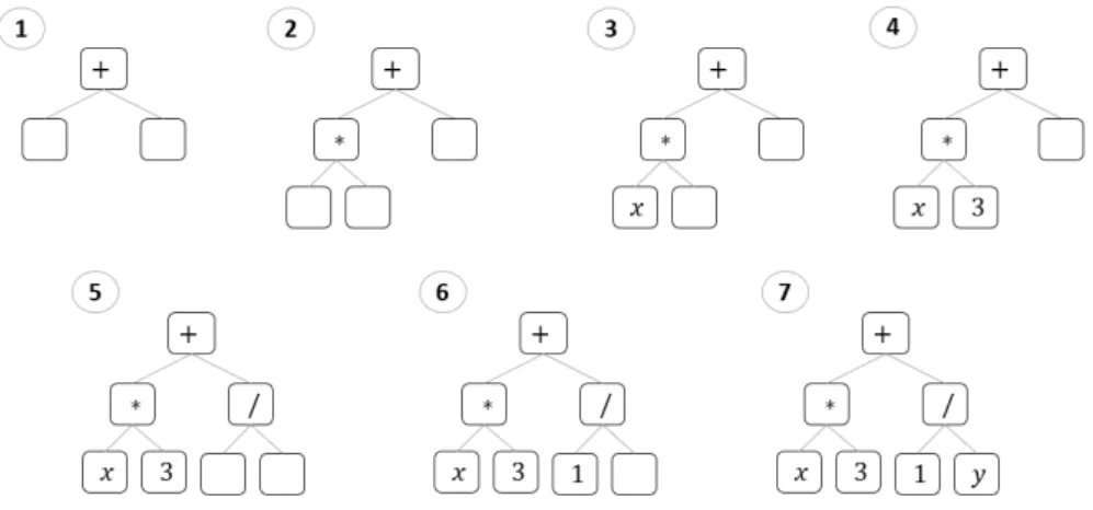
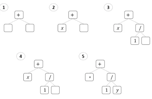
The initialization is a process of creating a set of individuals. In Genetic Programming an individual is a computer program expressed as a syntax tree, which consists of Terminals and Operators. Terminals are either variables or constants declared by the user. Operators are arithmetic functions that operate on the Terminals. Together they form Primitives Set, from which each tree is composed.

The individuals for the initial population are generated randomly. How-ever, researchers has identified various approaches for creating the initial pop-ulation. The most common approach is a mixture of two basic methods: full

(27)

and growth. In each situation the individuals are created till the specific max-imum depth of the tree, specified by the user. In specific cases, when the user knows the properties of an expected solution, the part of a population can be seeded with the trees having these specific properties.

Full method

The main principle of this approach states that all of the leaves in a tree need to have the same depth. It means that until reaching the maximum depth, the nodes of the tree are selected only from Operators set, while at the last level, there are selected only Terminals. The example of this process is illustrated on a figure 3.1.

Figure 3.1: Example of a tree generation process using full method The population created with this method is composed by trees that are very robust and have a large number of nodes. Although it doesn’t mean that each tree looks exactly the same and has the same number of nodes. As Operators can have different arity. The most common arithmetic functions have arity equal to one or two, and sometimes there can be more compound functions like if-else expression. Therefore trees built with this method will always have the same depth, but not necessary the same number of nodes.

Growth method

There is one major difference between full and grow method. In the first approach nodes were selected only from Operators set until reaching the max-imum depth of a tree. In the second approach nodes are selected from the whole Primitives set. If the Terminal is chosen, grow of the branch is stopped. Therefore the length of branches in a tree may differ. As a result, the trees in a population generated with this method are less robust than in the previous

(28)

case and have smaller number of nodes.

Figure 3.2: Example of a tree generation process using grow method Ramped half-and-half method

Neither full nor grow method is sufficient for initializing the population with individuals in variety of shapes and sizes. As a solution for that problem the new approach was introduced by Koza (1992). The proposed solution was to initiate half of a population using full and half using grow. In addition to that the range of maximum depths is used. By doing so, the variety of sizes and shapes of individuals is assured.

3.3 Selection

As the initial population is generated, the process of evolution begins. In order to ensure that good individuals are generated in next generations, the genetic operators are applied to the individuals selected based on fitness. Parent pro-grams with high fitness are more likely to generate good solution. Therefore few methods of selection based on fitness were introduced. Although the main approach is to select only good trees, there has to be a possibility of selection for every single tree. Week trees have smaller probability of being selected, but there is a chance given to them to improve themselves.

(29)

Tournament Selection

In this approach, the random sample of individuals is selected and their fitness values are compared. The one with the best fit is selected for to be a parent. This method does not require calculation of how good is the solution in com-parison to others, it just takes the best one in a sample.

Fitness-proportionate Selection

On the opposite to the previous method, this one takes into a consideration not only the fact that one individual is better than others, but also how good it is in comparison to others. In order to calculate the probability of selection for each tree, the fitness values of individuals in a whole population are calculated. Then the sum of the probabilities, 1, is divided between solutions proportion-ally according to their fitness. This method is also known as a roulette-wheel selection.

Ranking selection

The last method is very similar to the previous one. The only difference is that in this case, the probability is calculated proportionally to the place that a specific solution takes in a ranking of all individuals in a population. It is a good solution in cases when there is one solution with much higher fitness than the rest. In previous method this individual would have very high probability of selection, dominating the others, while in this approach the probabilities are distributed more evenly.

3.4 Replication and Variation

Once the parents are selected, the genetic operators are applied. There are 2 strategies that can be executed. Firstly, the individual can be moved to the next generation without any modification, in a process called Replication. Or secondly they can be selected for Recombination. Genetic operators are applied to the solutions with a specific probability. Therefore the situation when none of them will be applied, is possible.

In addition to that, there are methods of using replication in order to protect the best individual in a population. This method is called Elitism. As the selection and then all genetic operators are applied randomly, there is a chance that a good individual will not be selected and will not be present in the next generation. The goal of evolution is to find the best individual, hence protecting the best one in a population is reasonable and according to the research gives good results. As stated in the article written by Chang Wook Ahn and Ramakrishna (2003), the algorithms with elitism outperforms the standard implementations of GA. It is also shown how different versions of

(30)

this concept perform by means of an experimental study and it is stated that by using elitism the quality of the solution, as well as the convergence speed are improved.

Recombination is the process of modification of a solution by means of Crossover and Mutation. The purpose of these operators is to introduce to the population new individual based on the solutions selected in the first step.

Crossover

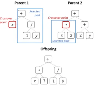
Figure 3.3: Example of subtree crossover

The most common form of crossover is a subtree crossover. After two

parents are chosen, there is a selection of a crossover point. It is done randomly, separately for each parent. Then the child is created by a copying the first parent until the crossover point and replacing a subtree rooted in that point by the part of tree starting in a crossover point of the second parent. The implementation of this genetic operator uses copies of individuals in order to allow a solution to be selected multiple times and produce more offspring. There are many specific forms of crossover and the particular versions used in the experimental will be specified in the next chapter.

Mutation

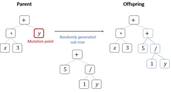
The purpose of mutation is to introduce in a solution small change in it’s ge-netic material. The most common methods are subtree and point mutations.

(31)

Figure 3.4: Example of subtree mutation

First one, similarly to crossover, selects a mutation point in a tree and re-places the subtree with a randomly generated one. It can be also described as a crossover between an individual and a randomly generated tree. An-other popular method is point mutation in which a randomly selected node is replaced by another operator or terminal from the primitives set. The only restriction in this approach is to replace node with another one, that has the same arity. As the described process is introducing rather small change to the individual, there was added a possibility of applying a mutation to more than one node in a single execution of this genetic operator.

3.5 Applications

Genetic Programming was proven to be successful in various data mining projects. The application of this concept in a classification problem was widely investigated by researchers. As discussed in an article by Chaudhari et al. (2008), GP can be applied to a multi-class problem. In that case, for each class a classification tree was built. The authors of the article are bringing up various applications of Genetic Programming. It is present in data mining, biotechnology, optimization, image and signal processing, computer graphics or even in electrical engineering circuit design.

As stated in the article by Espejo et al. (2010) describing the various appli-cations of Genetic Programming to Classification problems, GP programs were proven to be flexible and powerful. Mentioned article provides a summary of the research being available in this area. The main advantage of GP, according to article, is its flexibility. The process of evolution allows user to adapt this technique to the particular case by modifying building blocks of GP evolution. The domain knowledge can be applied by means of non-random initialization

(32)

or selection and definition of operators used for evolution. In addition to us-ing GP for development of an individual - a classifier, GP programs can be applied to perform feature selection and extraction. Feature selection is very important in Machine Learning tasks as it reduces the size of an individual and improve its interpretability.

An interesting example of modifying the core elements of Genetic Program-ming is presented in an article by Bojarczuk et al. (2001). The project was designed to understand the classification rules for diagnosis of certain medical cases. In order to do that, the primitives set was constrained to only logical and relational operators and variables from the database. Models created with this setting were tested on 3 different datasets connected to the field of medical studies. As the result, the rules detected by GP were more accurate than ones created by Genetic Algorithm or Decision Tree, proving the explanatory power of Genetic Programming.

In addition to wide application of GP in classifications problems, multiple articles confirm it’s successful implementation in various fields and problems definitions. As described in the article by Orove et al. (2015) in which the authors are using an evolutionary algorithm to predict student failure rate. It attempts to improve the student’s performance by detecting the students with problems and reducing the number of students who failed. The challenges that were faced by GP were large number of features, unbalanced dataset and lack of interpretability of currently used solutions. The researchers concluded that Multi-Gene Genetic Programming was able to evolve the model that accurately predicts student failure rates in few generations - 30.

Another interested use case was proposed by DANANDEH MEHR and

S¸orman (2018). The objective of the authors was to analyze the daily flow and

suspended sediment discharge that affect the hydrological ecosystem, especially during the floods. The state of the art for these analysis was use of Artificial Neural Networks. Developed models help with rivers engineering, as well as with planning and operation of river systems. Although the model that is being developed have to be complex due to the high variation of daily flows variations, in the article it is stated that Linear Genetic Programming can outperform Deep Neural Network Models and provides a model that achieves good performance.

Evolutionary Algorithms can be applied not only to different business areas, but also to various purposes. In papers published by Sehgal et al. (2019) and Such et al. (2017) it is showed how Genetic methods can serve as an optimization engine. It successfully explores the search spaces, that might be difficult to explore by standard search algorithms or are to complex to search it with exhaustive search. The biggest advantage of using GA for optimization of the Reinforcement Learning performance is the speed of finding the suitable

(33)

solution and good performance at chosen task. Also in the second article it is presented that the weights of Deep Neural Network can be evolved by using a simple population-based genetic algorithm, proving that it is possible to train neural networks with methods that are not based on gradient search.

To summarize, we can see that Evolutionary Algorithms as a method of optimization, and then Genetic Programming as its sub-type can be proven to be successful in various problems. These methods characterize with high pos-sibilities of customization of algorithms building blocks (methods) e.g. Seeding initial population with pre-trained individuals, specifying very restricted prim-itives set or enhancing the evolution process with newly developed cross-over and mutation methods. As a main objective of this research is to check if they are also fit to predict the errors of a predictive model, serving as a secondary point of performance verification and explanation.

(34)

(35)

Chapter 4 Experimental study

The objective of this chapter is to present the implementation of proposed research with use of Genetic Programming. Firstly we present the general description of the project - the logic of transforming an idea into the solution that can be executed, validated and applied to real problems. In this section we are providing the details of the research methodology and prepared test cases. For better understanding, we provide specific description of both, the predictive models and datasets used in the study. The research is based on three datasets with different number of observations and type of features for better analysis of the performance. All problems are classification tasks and contains predictions produced by four models, selected for this study: Logistic Regression, Decision Tree, Random Forest, Neural Network. Therefore the objective of the study is to train and test 12 independent programs.

Secondly we present details of the Evolution Process. As the parameters set up may be different for each of the models, it is important to present differences in the implementation. We state here some of the key decisions that were made during training process, e.g. selection of elements in primitives set or fitness function. For each test case we summarize the parameters of GP Algorithm that were used for final runs. Furthermore, the evolution process is documented and the results of study are summarized and analyzed. For that purpose we analyze the logs of training stage and the scores obtained by the best models on test and validation sets. Finally we draw general conclusions based on data.

As a technical note, most of the work was developed in Python ming Language (data preparation, generating predictions, Genetic Program-ming setup and evolution, summary of the results). Beside of the standard python libraries (e.g. numpy, pandas), predictive models were fitted and tested using Scikit-learn Pedregosa et al. (2011). This library provides a lot of data transformation, model management and validation functions, making the pro-cess of training the test models simpler. For the evolution of Genetic

(36)

Pro-CHAPTER 4. EXPERIMENTAL STUDY

grams we used DEAP package Fortin et al. (2012). It is the main tool in this research. The main part - the development of an algorithm was done using standard DEAP functions customized slightly to the needs of the project. Both libraries are enabling users to create prototypes of Machine Learning Models or Genetic Programming by using standard methods as building-blocks as well as enabling high customization possibilities.

4.1 Research Methodology

In this section we present the way of implementing the research idea that was proposed at the beginning of this thesis. First we present the general description of the project and use of Genetic Programming for this research. Secondly we describe how the process of generating predictions and developing a GP program is defined and how it is tested and analyzed in order to provide indications on the performance of developed models.

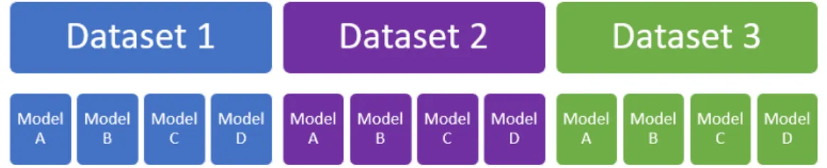
Furthermore, we describe the test cases used in this study. We start with machine learning models that were used for generating predictions, then we present selected dataset for training and testing these models. The datasets were selected in a way that assures differentiation in terms of types of variables and size of the dataset. This allows us to conclude on the generality of the approach. In total GP was tested on 12 test cases, being the combination of 4 predictive models and 3 datasets, what we can see on the diagram 4.1

Figure 4.1: Visualization of the test cases preparation

4.1.1 Data Flow in a project

In this section we describe the structure of the data splitting and processing that we perform for each of the test cases. The full flow is illustrated on the figure 4.2. As the first step we load the dataset and split it into train and test set. Specific datasets chosen for the research are described in the next chapter. After a dataset is divided, the training data is used for fitting selected predictive models, while test data is used for generating predictions

(37)

CHAPTER 4. EXPERIMENTAL STUDY

and will be the input data for Genetic Programming application. The outputs of fitted models calculated on test data are compared with the target labels. Then we create a flag that will indicate if specific prediction was wrong or correct. We flag errors with value ’1’ and keep 0 for correct predictions. This flag is used as a target variable in the GP development.

In the second stage of the project - the main phase - we use test data from previous step and split them into train, test and validation sets for training and evaluation of GP Program. On the first, biggest part of the data we evolve a model, that is then tested on test data for assuring the lack of overfitting and evaluated on validation set. The final validation is done on the unseen data as it is done on real-life project for assuring the stability of models.

Figure 4.2: Datasets transformations used in experimental study and steps applied in the process.

4.1.2 Predictive models used in the study

In this section we summarize all machine learning models that were used in the study. Decisions made by those models on datasets used in the study will be a subject to evaluation done by GP Program. There are selected different types of models for generalization purposes. First we present an linear model that is widely used for classifications problems, then we present model based on if-else rules and one that is an ensemble of many weak classifiers, finally presenting a model that is a basic version of popular Deep Learning Models.

(38)

Logistic regression

A binary classification model that is based on a concept of odds ratio, which is calculated based on a probability of an event that is being predicted. The odds ratio can be calculated with a formula: p/(1 − p), where p is probability of this event. Then the result is passed to a logarithm function that’s trans-form the ratio into a range of values in order to fit a linear regression with the input features, that in this case is called logit. The learning algorithm is approximating the coefficients of the regression mentioned in the previous step. In order to calculate a probability of an event, a value obtained from fitted model is transformed by an inverse of a logit function. It is calculated

with the formula: 1/(1 + e−z), where z is the result from regression, and this

function can be called logistic or sigmoid - due to its shape. Decision tree

A model represented in a shape of a tree that is represented as set of if − then − else rules. In contrast to the previous algorithm in this case there are no weights to be fitted by an optimization algorithm. The learning is done in a sequential way by dividing training dataset into subgroups according to a selected measure. One of those measures is entropy, which calculates the disorder of a subset with respect to the output label. The algorithm to create a decision tree starts with calculating a value of selected measure, selecting a variable with best value to be the first rule to create subsets - leaves. The main advantage of this algorithm is his interpretability, as we can easily read the rules that exist in a dataset from the tree form. On the other hand, while fitting decision tree there is a high risk of over-fitting (creating a model to well explaining training data and with poor generalization capabilities).

Random forest

It is a method of creating a good model by combining a set of week classi-fiers, typically decision trees. It is widely used by a community due to the fact that it has good performance, scalability and the fact that it is resistant to the problem of over-fitting. It consists of a number of trees. Each tree is fitted with the method described in the previous chapter, but with restricted dataset. The dataset used for each classifier has randomly selected features and observations in order to create model that are specialized in some portion of the data. As a result we obtain a number of predictions, one from each tree, and we aggregate those by majority voting.

(39)

Perceptron

The inspiration for creating this algorithm was a nerve cell in a brain that is transforming signals (inputs) into other signals (outputs), that are passed to the next cell. The brain is able to learn by allowing its cells to communicate with each others passing on and transforming information. This concept was first introduced by McCulloch and Pitts (1988) and then developed as per-ceptron learning rule by Rosenblatt (1957). Perper-ceptron is a model in which there is one or more neurons, but they are arranged in a single layer. This means that there is no situation in which output from one unit is directly passed to output layer, not to another unit. Additionally, information in units is passed in one direction - from inputs to output, and inputs are connected to the main cell by means of randomly generated weights. During learning process an algorithm tries to adjust the coefficients in order to make correct predictions.

4.1.3 Dataset Used in a Study

In this section each of the test cases is described. To begin with, we pro-vide the overall summary of the data, focusing on the number of observations and types of features. Then we summarize the prediction generation process and calculate accuracy scores for each of the models fitted on a test dataset. Eventually we describe the settings for the evolution of the GP programs.

In order to test GP programs on different sets of data, the test cases for experimental study are selected with respect to different data types and num-ber of errors in the predictions on test set. First we select a small dataset with high accuracy in order to test if GP is able to identify errors based on a small number of samples. Then we select a larger dataset that contains numeric variable as well as categorical. Additionally, the models fitted on this dataset have low accuracy. By doing so, we can test how programs are performing on a different types of data and how they operate when there is more errors in a prediction. Finally we select large dataset with high number of numeric variables to check how the programs are going to perform on large number of inputs and different accuracy scores.

Any required data transformation is described in each of the test case de-scription. Additionally as one of the test cases contains categorical variables, we applied in that case encoding of the categorical columns into series of bi-nary features. Genetic Programming does not work correctly with missing data, therefore as a safety precaution, if there are any missing data in the input dataset, we replace them with Median of a column.

(40)

Test case 1: Breast Cancer Wisconsin

First test set used to conduct the experiment is Breast Cancer Wisconsin (Diagnostic) Data Set (1995) hosted by Machine Learning Repository created by University of California, Irvine.

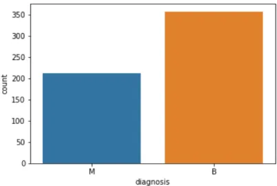
In the data there are 569 observations and 30 features, plus one column with target label with 2 levels: B for cancer being benign and M for malignant. All of the explanatory variables are numeric, which is good for the performance of the Predictive Models and Genetic Programming. The count of values for each class in dependent variable is presented on the Figure 4.3. It appears to be slightly skewed (63% of observations being benign), but there is no need for an adjustment in form of down- or up-sampling.

Figure 4.3: Distribution of dependent variable in Breast Cancer Wisconsin dataset

The dataset was partitioned into training and testing set, with the 60% of observations being in the test set, which stands for 342 records. Usually, good practice is to have 70% of observations in the training set and only 30% in test set, but as the research is done on the test set, it is important to have there enough observations to train GP program. To assure good representation of positive class in the test set, the division was done stratifying the sample by target label. Four predictive models were fitted on the training set and their performance on the test set was summarized in Table 4.1.

(41)

Test case 2: Bank Marketing

Second test set is related to direct campaigns of a Portuguese banking institu-tion and the data about clients subscribing to a term deposit Bank Marketing Data Set (2012). Similarly to the previous case this dataset is also listed on Machine Learning Repository created by University of California, but in the test study we use a copy hosted by Kaggle platform.

Marketing campaigns were executed by calling potential clients. The clas-sification task in this example is to predict if the client will subscribe to the term deposit after presenting the offer or not. The information is coded in variable y: yes (1) - if client subscribed for the deposit, no (0) - if this did not happen. In the provided dataset, there are 16 explanatory variables. 9 of them are categorical and the rest of them is numeric. For the discrete features we perform transformation into binary labels in order to fit all predictive models correctly. Therefore in a final dataset there is 51 numeric columns.

Dependent variable is well balanced. The comparison of observation count in each class is summarized on the figure 4.4. Within the 11162 observations,

Figure 4.4: Distribution of dependent variable in Bank Marketing dataset there are 5873 cases when customer did not signed for a deposit and 5289 when the marketing campaign was successful. The percentage of positive cases is equal to 47% and therefore there is no need for down- or up-sampling.

The dataset was partitioned into training and testing sample with the 60% of observations being in the test set, which stands for 6698 records. Division was made taking into account similar distribution of y in both sets. Four pre-dictive models were fitted on the training set and their performance on the test set was summarized in Table 4.1.

(42)

Test case 3: Polish Companies Bankruptcy

The third data sets contains information about polish companies with an indi-cation about it’s bankruptcy. File is hosted by Machine Learning Repository created by University of California, Irvine Polish companies bankruptcy data Data Set (2016). The data was collected from Emerging Markets Information Service. The analysis of companies bankruptcy was analyzed over a period of time. The bankrupt companies were evaluated from 2007 to 2013, while operating from 2000 to 2012.

For the purpose of conducting experimental study, we select the data from first year of the forecasting period and corresponding target label that defines the bankruptcy status after 5 years. In the dataset there are 7027 observations and 64 features plus target label. All of the exploratory variables are numeric. Target label has two values: no (0) - if company still operates and yes (1) - if company went bankrupt. Unfortunately the positive class is not represented enough in the dataset. There is only 0.04% of ones in the target label. There-fore we perform up-sampling and raising the value to 50%. The comparison of observation count in each class, before and after transformation, is represented on the figure 4.5.

Figure 4.5: Distribution of target variable in Polish Companies Bankruptcy dataset before and after up-sampling

Additionally, there are missing values in the dataset. In order to assure better performance of predictive models and successful run of GP evolution the observations containing missing values need to be excluded from a dataset or

(43)

have these values replaced with some logic. In this study we use f illna method from pandas.DataF rame and as a logic we use replacement with median of a column.

The dataset was partitioned into training and testing sample with the 60% of observations being in the test set, which stands for 6698 records. Division was made taking into account similar distribution of y in both sets. Four pre-dictive models were fitted on the training set and their performance on the test set was summarized in Table 4.1.

Summary of the Test Cases

In the table below we can see the summary of the Predicted Models trained on the test cases. For each of 3 datasets there are 4 models trained and tested. In the table below we can see how Accuracy varies between different test cases. The average accuracy here is 80% and it varies from 59 to 98 percent.

Test case Model Accuracy Errors Observations

in a test set Breast Cancer Wisconsin Logistic regression 95.03 % 18 342 Decision tree 93.27 % 23 Random forest 94.74 % 18 Neural network 75.44 % 84 Bank Marketing Logistic regression 82.32 % 1184 6698 Decision tree 76.93 % 1545 Random forest 79.90 % 1346 Neural network 68.23 % 2128 Polish Companies Bankruptcy Logistic regression 75.48 % 1988 8108 Decision tree 79.43 % 1668 Random forest 98.36 % 133 Neural network 59.46 % 3287

Table 4.1: Summary of the predictions used as test cases

All test sets used for evaluation of the predictive models were saved and are used in GP experiment as input datasets. Additionally the errors are calculated for each vector containing predictions of a given model, on given dataset. We mark the errors with a flag: (0 if prediction was correct, 1 -indicating an error ). This flag will serve as a target variable in the next step of the process. In the table 4.1 we summarize all 12 test sets with the accuracy

(44)

of a specific model. We can see how good was the prediction that is going to be evaluated and what is the size of the set. Additionally we provide the number of incorrect predictions, that we want to detect with use of Genetic Programming.

4.2 Experimental settings

In this chapter we explain how the study was prepared and guide through all the steps that lead to the results presented in the next section. We summarize briefly input data and the code structure for a Genetic Programming execution. Starting from general overview of applied steps and methods for initialization and variation phases to detailed summary of the settings used in each of the test cases.

As mentioned in the introduction to this chapter we are conducting the research using python programming language and library: DEAP. This tool gives a lot of freedom while setting up a simple GP run. The code withing the package can be easily customized and enhanced.

Firstly, let’s discuss the logic behind whole process. The idea is to take the predictions of the statistical model, for each of the observation check if the prediction is the same as target label and train a GP program that detects errors. It is explained by a diagram on figure 4.6. The input datasets for GP evolution are test sets from the previous step. The target variable that is being predicted is calculated by comparison of predictions of machine learning models with the original labels. The input sets are fed into an algorithm and the output is transformed by logistic function in order to obtain the probability score for each observation. The vector of probabilities calculated at each generation is used for evaluation of individuals and the selection for variation step.

As additional step of the process we transform the vector of probabili-ties into binary variable containing the decision of selected model by simple threshold. If probability returned by GP individual is higher than 0.5, then the decision is that the prediction was incorrect (value : 1), otherwise the Ma-chine Learning model was right and we assign value : 0. This vector is used for calculating conventional Accuracy as a second step verification. It is done by comparison of the confusion matrices generated by different models.

There are 3 data sets and for each dataset, there are 4 models applied. This means, that there are 12 different test cases in which we need to train and evaluate the GP program. In the research we want to assure that the results we obtain are general and valid despite of test case. Hence we are using data of different format (numeric and categorical variables), different statistical models (Logistic Regression, Decision Tree, Random Forest, Neural Network ) with various accuracy. The best model that is being examined has

(45)

Figure 4.6: Implementation of the research idea

almost 99% of accuracy, while the worst one has 59%. It allows to asses the performance of the models on well-fitted models as well as on close to random classifiers.

The input that is being processed by GP algorithm consists of test set -on which we generated predicti-ons in the previous step, and array c-ontaining information if the prediction was correct or not. It is represented on Figure 4.7.

Figure 4.7: Data split conducted in the project

After data is loaded into python environment we secure 15% of the data for final validation of the model and call it validation set. The remaining data is divided into train test and test set 10 times for 10 runs of an evolution process. Programs in GP algorithm are using only train set for learning. The test set is used at the end of each run to evaluate the best individuals in the final population. As a performance measure of the final model we apply the best

(46)

individual of all runs to the unseen validation set and calculate the accuracy of prediction.

Moving forward to the implementation of Evolutionary Algorithm in this research. DEAP library provides multiple methods for initialization and vari-ation (cross-over and mutvari-ation). In all of the test cases the initializvari-ation of a population is done using Ramped half-and-half method, where half of popula-tion is created using method grow and half is created with full method. The set of available functions and terminals for initialization is stored as a primitives set and contains:

• Terminals

Inputs: All explanatory variables present in the input data

Constants: (−1, 0, 1)

Floats: (0.1, 0.2, 0.3, 0.4, 0.5, 0.6, 0.7, 0.8, 0.9)

Integers: (2, 3, 4, 5)

Booleans: T rue, F alse

• Functions

Basic mathematical: +, −, +, /

Numeric Functions: negative, sinus, cosinus

Boolean Operators: and, or, not, if − then − else

The Primitive Set contains building blocks for creation of the Programs. The most important element of this set is the set of input features. These are the explanatory variables from the datasets mentioned in the previous chap-ter and their number varies from 30 to 64. Due to the fact, that there are both only-numeric or mixed-typed datasets, we introduce to the set functions and operations that are fitted to work with categorical variables. Therefore in Terminals, we introduce booleans: true, f alse and logical functions mentioned above. There are also introduced some constant values, serving as parame-ters in evolved individual and numeric functions allowing transformations of numeric inputs, like trigonometric functions and negative sign. In addition to basic mathematical functions, we transform division by adding syntax pro-tecting it to divide by zero and return an error and call it protected division. Remaining functions operate correctly on the numeric and binary scales, there-fore no additional transformation is needed.

Fitness Function

After population is created, there is time for evolution. In each generations the individuals are evaluated using the fitness function implemented for this

(47)

project. Selection of the correct method to evaluate programs is a crucial part of training of the machine learning model. It allows to select a model which is not only well-fitted to training data, but provides good generalization abilities that can be applied to test and validation sets.

The most conventional method for evaluation of machine learning models is simple accuracy. It summarizes the percentage of correctly classified obser-vations. It is calculated based on the values presented in a form of confusion matrix, in which predicted outputs are compared to real labels. Although it provides good overview of the predictions, it is highly biased in some of the cases. For instance, if the models is very successful and only 3% of all ob-servations are classified incorrectly, then by creating a model that will assign ”0” to all records, we will achieve accuracy of 97%. It is a valid point for all imbalanced problems.

As an alternative method of evaluating a solution, we propose Area under ROC (Receiver Operating Characteristic). It was studied by Bradley (1997) and discussed in their paper from 1996, that AUC - Area under Curve can serve successfully as an evaluation of models. It is concluded in the paper that this method can be used for single number evaluation of ML models and provides the evidences, that is improves the visibility of the predictions as well as the performance. The starting point for calculating an area under ROC is also confusion matrix. The data that are summarized there in 4 categories: true negatives, false negatives, false positives and true positives. While conventional accuracy summarizes only true negatives and true positives, in ROC curve we can observe how true positive rate and false positive rates are changing for different threshold values. The details of this fitness function together with its application to the signal detection theory and analyzing the trade-off between hit rates and false alarms is presented in the article by Vuk and Curk (2006). The result of the research was that by using Area under ROC the classification accuracy can be improved and this statement was validated on several test cases. This fitness function can be calculated on the vector of probabilities. In order to do that, we apply the logistic function to the output generated by GP as showed on figure 4.6. By generating the vector of probabilities we allow model to fit to the general rules in the dataset, not only data in training set.

In the table 4.2 we can see two examples of the models evaluated on vali-dation set prepared for one of the test cases mention in previous section. We can see observe how model evolved with Accuracy as a selected evaluation method and how a model with area under ROC performed. We can see that by using simple accuracy we may faced an issue of singe value prediction. In this case model is predicting all classes to be 0, so it does not satisfy the task, which is errors detection. On the right side of the table we can see that with second fitness function, the numbers are more trustworthy, as the prediction