REVISTA DE M ´ETODOS CUANTITATIVOS PARA LA ECONOM´IA Y LA EMPRESA (25). P´aginas 3–22. Junio de 2018. ISSN: 1886-516X. D.L: SE-2927-06. www.upo.es/revistas/index.php/RevMetCuant/article/view/2312
Destabilizing Impacts of Herding Behaviour in
Portuguese Capital Market
Marques Leite, Gabriela Department of Management
Research Centre for the Study of Population, Economics and Society Lusofona University of Porto (Portugal)
E-mail: gabriela [email protected]
Machado-Santos, Carlos
Department of Economics, Sociology and Management University of Tr´as-os-Montes and Alto Douro (Portugal)
E-mail: [email protected]
Ferreira da Silva, Am´elia Institute of Accounting and Administration Centre for Organisational and Social Studies
Polytechnic Institute of Porto (Portugal)
E-mail: [email protected]
ABSTRACT
The present work seeks to analyze the herding behavior phenomenon as a destabilizing factor of the capital market, while studying the relation between the herding behavior phenomenon and market profitability and volatility. The results allow us to verify the existence of a significant inten-sity of herding, especially when price variation occurs. Conversely, asym-metrical and elevated volatility levels ensue, with a higher probability of profit than losses of the same magnitude. However, results are less visible when one looks at the causality relation between herding and market volatil-ity. This paper contributes to a deeper understanding of herding behavior and its relation with market efficiency.
Keywords: Herding behavior; behavioral finances; volatility; capital mar-kets; investors’ rationality.
JEL classification: 91G50. MSC2010: 62G08; 62G10; 91G70.
Art´ıculo recibido el 4 de diciembre de 2016 y aceptado el 21 de junio de 2017.
Impactos desestabilizantes en el comportamiento
gregario en el mercado de capitales portugu´
es
RESUMEN
El presente trabajo busca analizar el fen´omeno del comportamiento gre-gario como un factor desetabilizante en el mercado de capitales, estudiando la relaci´on entre el fen´omeno del comportamiento gregario y la rentabilidad y volatilidad del mercado. Los resultados nos permiten verificar la existencia de una intensidad significativa de gregarismo, especialmente cuando tienen lugar variaciones de precios. Rec´ıprocamente, sobrevienen niveles elevados y asim´etricos de volatilidad cuando hay mayor probabilidad de beneficios que de p´erdidas con la misma magnitud. Sin embargo, los resultados son menos visibles cuando se observa la realidad de causalidad entre gregarismo y volatilidad de mercado. Este art´ıculo contribuye a una comprensi´on m´as profunda del comportamiento gregario y su relaci´on con la eficiencia del mercado.
Palabras claves: comportamiento gregario; finanzas conductuales; volatil-idad; mercado de capitales; racionalidad de inversores.
Clasificaci´on JEL: 91G50.
MSC2010: 62G08; 62G10; 91G70.
5
1. Introduction
Capital markets are constantly changing and, especially in recent years, were faced with several situations that test the strength of the financial system, and its regulation and the supervision mechanisms. The new millennium began in a recessive economic climate and high market volatility, resulting, among other factors, from the speculative movement of the 1990’s. A permanent price increase culminated with the bursting of the speculative bubble in 2000. Several authors attributed to the herding behaviour as an important cause to the instability of the markets, justifying it is responsible for the creation of price bubbles. Herding behaviour is about investors decisions to replicate of others investors or follow market consensus rather than based on their own beliefs and information.
The aim of this study is to analyze the herding behaviour as a potentially destabilizing factor in the Portuguese capital market between 1998 and 2010. Accordingly, this work has been developed in three lines of research, namely: (i) determining the intensity of herding present in the market; (ii) estimating the effect of various intensity of herding measures on market volatility; (iii) study of the impact of herding in market profitability.
2. Literature review
In financial markets, herding behaviour has been identified for some time (Jain and Gupta, 1987; Bikhchandani and Sharma, 2000) and everywhere (Filip et al. 2015; Lugo et al, 2015; Tan et al, 2008). There is a strong believe that “investors are influenced by the decisions of other investors and that this influence is a first-order effect” (Devenow and Welch, 1996: 604). But, to which extension herding behaviours are rational or irrational? This is not an easy question. Indeed, investors are subject to sentiment, their behaviours are complex (Baker and Wurgler, 2007, Baker et al, 2012) and “some phenomena that seem irrational can actually arise very naturally in fully rational settings” (Hirshleifer and Teoh, 2001:2).
Literature on behavioural finance provides several explanations for this phenomenon. Bikchandani et al. (1998) suggest that investors obtain information by observing other investors’ transactions, and adopt the same investment strategies. On the other hand, Hirshleifer et al. (1994) consider that herding behaviour is mostly present because investors tend to pursue the same information sources and, as a result, they interpret the signs in the same fashion which translates to similar interactions in the market. Other authors list as causes for herding behaviour the so-called reputation costs [e.g., Scharfstein and Stein (1990), Trueman (1994)] and compensation schemes [e.g., Roll (1992), Rajan (1994), Maug and Naik (2011)]. In turn, Gompers and Metrick (2001) argue that herding behaviour can arise if investors feel attracted to assets with similar characteristics.
Lastly, several authors point out as causes for herding behaviour the degree of institutional participation in the capital market, the quality of information issued, opinion dispersion, turnover, market size and degree of sophistication (e.g., Demier and Kutan, 2006; Henker et al., 2006; Patterson and Sharma, 2010; Puckett and Yan, 2008).
Broadly speaking, the informed trader theory acknowledges that if institutional investors are seen as particularly astute or well informed, their purchases and sales tend to be taken as informative signs on fundamental economic variables (or about the future equilibrium of asset prices) by less informed investors (or noise traders), the latter which are likely to invest in the same way as the former. Therefore additional purchases (sales) by institutional investors would provide evidence that asset prices would be below (above) their actual value, and hence other investors, noise traders, would tend to trade in the same manner as institutional traders, inducing pressure for more prominent price increases (decreases). This second phenomenon, known as herding behaviour, is thus seen as a contribution for asset price instability. This phenomenon is nothing more than the adoption of a similar strategy, the imitation of other investors (in this case, institutional investors), ie
6
buying and/or selling the same assets in the same moment in time (e.g., Friedman, 1984; Lakonishok et al.,1994).
Alevy et al. (2003) argue that in an economic environment where investors possess imperfect information about the true state of the capital market, it may be a rational attitude to ignore the very information they have and choose to make investment decisions based on what they believe to be public information signals. Herding behaviour occurs precisely when investors knowingly make identical choices concerning the purchase and/or sale of an asset at the same moment in time, despite the fact that they possess information that would lead them to trade in another manner. Many investors acquire their ideas about financial markets from other people, whether through newspapers, television or analysts' opinions, without even verifying whatever variables relate to that. They possibly think “Who am I to verify? These people are supposedly the experts on the subject.” In fact, many investors are emotionally dependent on that type of information that, in truth, doesn’t provide more insight than the short-term decisions of other investors. It may be argued that this type of dependency appears to be a universal trait, even in investors with long term prospects. They end up being driven to herd behaviours because they don’t possess "first-hand" information adequate to forming an independent belief, which causes them to start a incursion in search of wisdom through numbers. Their subconscious is telling them: “You have a too small knowledge base to make decisions by yourself, your only alternative is to assume the herd knows where it’s going (Pretcher, 2001: 121).
Several studies propose a variety of measures and indicators to attest the existence of the of the herding behaviour, including Wermers (1999), Chang et al. (2000), Hwang and Salmon (2004), Sias (2004), Patterson and Sharma (2010). Despite the convincing arguments about the herding behaviour are numerous and pointed, and even market watchers observe their occurrence, the empirical evidence is scarce and relative few cases confirm its existence (Blasco et al., 2009).
3. Database and methodology
3.1 Description of the Database
In order to assess the intensity of herding in the Portuguese capital market, the data are processed on a daily basis and over a time span of 144 months (12 years), between July 1998 and June 2010. Initially, the analysis focuses on the market index – Portuguese Stock Index 20 (PSI-20), and whenever it is possible to adapt the methodology; further tests are performed to the shares underlying the market index.
3.2. Intensity of herding Measure
The methodology adopted is in accordance with Blasco et al. (2009), and the intensity of herding estimated according to Patterson and Sharma (2010), measured both in sequences initiated by the buyer and in sequences initiated by the seller.
Based on the information cascades model by Bikhchandani et al. (1992), Patterson and Sharma (2010) report that an information cascade is noticed when negotiation sequences initiated by the buyer or the seller are larger than the negotiation sequences which would be observed if each investor decided only on the basis of the information they possessed. Thus, if investors systematically imitate one another, the statistical indicator values should be negative and statistically significant, in that the actual number of sequences initiated is lower than expected:
7
x(i, j, t) =
(r + 1 2) − np (1 − p )
⁄
√n
(1)
Where: ri = real number of type i sequences (high, low or neutral); n = total number of transactions performed in active j on t day; ½ = adjustment by discontinuity parameter; pi = probability of coming across an i type sequence.
In asymptotic conditions, the (i, j, t) statistic follows a normal distribution of zero mean and variance:
σ (i, j, t) = p (1 − p ) − 3p (1 − p ) (2)
Therefore, Patterson and Sharma (2010) define the intensity of herding measure using the following statistic:
H(i, j, t) =
x(i, j, t)
σ (j, t)
. .
N(0,1) (3)
The i variable assumes three different values, depending on the type of transactions mentioned above, so as to obtain Ha, Hb and Hn statistics for every day and for every title underlying the market index.
3.3. Measures of volume, volatility estimates and herding
The volatility of asset prices is a factor of paramount importance, first because it provides the basis for both the models of price formation and their own risk management strategies. According to the theory of market efficiency, volatility is explained solely by the automatic process of price adjustment to new relevant information conveyed to the market. However, the process of forming asset prices, and hence the actual volatility are not uniquely dependent on available information but also on a number of other aspects, such as the psychological decision processes of the investor himself. In this sense, the herding behaviour may occur in the capital market and, in some way, contribute to the increase in volatility and therefore to the destabilization of the market itself. Thus, in line with the stream of authors who believe that investor behaviour can have an impact on volatility, we estimated the effect of different levels of intensity of herding on the degree of market volatility. However, the (temporary) effect on the price of the large-block transactions and day-of-the-week is purged from the measures of estimated volatility, so as not to distort the results.
3.4. Volatility estimates
As a volatility measure, the absolute return residual allows us to assess the causal relationship between past performance and current returns. Therefore, we estimate the regression between the daily returns of asset j in the current period and the daily return of the asset j in the recent past (30, 90 and 180 days).
8
Where: Rjt = return of asset j on day t, which can take on four values: (1) AA if return is calculated using the opening prices of day t and day t+1, (2) AF if return is calculated using the opening and closing prices of day t, (3) FF if return is calculated using the closing prices of day t and day t-1 and (4) FA if return is calculated using the closing prices of day t and the opening prices of day t+1; Dkt a dummy variable, that adopts the value one for Monday and zero for the remaining days of the week; Rj,t-p = past return of asset j, where p=30, 90 or 180 days); │εjt│= vola lity measure for each series employed; jk and jk are the model parameters.
Given the possibility that the daily series of data may display a seasonal pattern, the model includes a dummy variable and regression is estimated by deducting this effect from the respective period. In this sense, the dummy variable is included in order to capture the differences in average returns that are exclusively derived from market performance on different days of the week and past performance is included in the model to counteract the autocorrelation between profitability series.
The estimates of historical volatility, are according to Parkinson (1980) and Garman and Klass (1988), employ the maximum and minimum daily rates for its calculation, as the authors consider that the extreme values of a session are more informative than the opening and/or closing prices. Hence, when prices reach extreme values they tend to revert to the medium that, in turn, not only assists the monitoring of extreme volatility but also allows a more correct prediction.
3.5. "Clean" series from the effects of traded volume and the day of the week. After estimating the volatility measures, absolute return residuals and historical volatility, it is essential to isolate the effects of turnover and day of the week. To this end, further regressions are estimated in which each measure of volatility described above depends on the day-of-the-week (including a dummy variable in the model) and an approximate measurement of the daily transactions volume (transactions volume in euro, number of transactions and average value of transactions in euros). Thus, after obtaining the residue of the estimated regressions, we obtained series in which the effects would be derived from factors other than the turnover of the day-of-the-week that, being present, would be seized by the coefficients of the variables considered.
In compliance with the method of Chan and Fong (2006) three measures of volume are used, namely: (i) volume of transactions in euro, (ii) number of transactions, (iii) average transaction value in euro. Given that the literature is divergent on which of these measures has greater impact on market volatility, the option was to test all, in order to obtain more feasible results. As such, the estimated regressions, using the OLS method are as follows:
σjt = αj+ αjmMt+ ρjkσjt−p+ ϕjVjt+ υjt nj k=1 (5) σjt = αj+ αjmMt+ ρjkσjt−p+ θjNTjt+ ηjt nj k=1 (6) σjt = αj+ αjmMt+ ρjkσjt−p+ γjVMTjt+ τjt n k=1 (7)
where: σjt = value of each volatility measure taken into account in day t, where j assumes the different values of the absolute return residuals estimates and historical volatility; Mt = dummy variable, that adopts the value one for Monday and zero for the remaining days of the week; Vjt = volume of transactions in euro of asset j in day t; NTjt =
9
number of transactions in euro of asset j in day t; VMTjt = average value of transactions in euro of asset j in day t; jt, jt and jt = residuals of the regressions which, after elimination of the effects of volume and day-of-the-week, comprise the new volatility series; j, jm, jk, ϕj, θj and j are the model parameters.
3.6. Effect of herding in volatility
Herding behaviour, as behavioural imitation of the strategies of other investors, may be seen as a destabilizing factor in the market, given the increased volatility that it can generate. Accordingly, after obtaining "clean" volatility series from the procedure described in the previous section, an analysis of the effect of herding in daily volatility must be done. For this, we use the following regressions, using the OLS method:
υjt = ωj+ Hijt+ λjt (8)
ηjt = ωj+ Hijt+ λjt (9)
τjt = ωj+ Hijt+ λjt (10)
Where: jt, jt e jt = residuals of expressions (5), (6) and (7); jt = model parameter; Hijt = intensity of herding measure on day t, where i assumes three different values, according to equations (1) and (2); and λjt = regression residuals.
These results could ascertain the extent to which the intensity of herding has an impact on market volatility.
3.7. Herding and profitability
The herding behaviour, as behavioural imitation between investors, may enhance the destabilization of asset prices [e.g., Friedman (1984), Lakonishok et al. (1994)]. As such, after analyzing the relationship between herding and volatility, it is important to examine the link between this phenomenon and profitability, through regressions (11) and (12):
Hijt = α1+ βkHij,t−p+ δkRj,t−p+ εt1 nj k=1 nj k=1 (11) Rt= α2+ ϕkHij,t−p+ γkRj,t−p+ εt2 nj k=1 nj k=1 (12)
Where: Hijt = intensity of herding measure, described in equations (1) and (2); Rj = daily profitability of the PSI-20 index; εt1, εt2 = regression residuals; and 1, 2, k, k, k and k are the model parameters.
Initially, we analyze the way in which past profitability and the intensity of herding in the past influence herding in the current period. Basically, we attempt to understand whether historical profitability conditions the intensity of herding. Later, we want to determine whether the intensity of herding or past profitability has an impact on index profitability.
4. Empirical analysis
4.1. Measure of Herding Intensity
With the purpose of determining intensity of herding in the Portuguese capital market, we applied the methodology of Paterson and Sharma (2006). Therefore, we calculated the daily return of the shares underlying the index, grouping by type a, b or n –
10
depending on whether the return obtained is positive, negative or zero, respectively. This procedure allows an identification of the real number of sequences by type, as well as the total number of daily transactions carried out per share, and thus complete the calculations proposed in the equation (3). Consequently, after calculating the average value of the transverse series and obtaining the resulting time series of average values, it is possible to assess the statistical series in sequences of high (Ha), low (Hb) and neutral (Hn), according to equation (4).
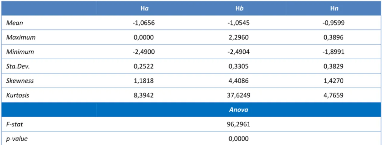
Table 1 presents some descriptive values of the intensity of herding measure, in sequences of high, low or neutral, which occurred in the shares underlying the market index for the period July 1998 to June 2010. The last two lines present the F-statistics (and their associated probability) for the null hypothesis of equality of means between series.
Table 1. Intensity of herding measure
Ha Hb Hn Mean -1,0656 -1,0545 -0,9599 Maximum 0,0000 2,2960 0,3896 Minimum -2,4900 -2,4904 -1,8991 Sta.Dev. 0,2522 0,3305 0,3829 Skewness 1,1818 4,4086 1,4270 Kurtosis 8,3942 37,6249 4,7659 Anova F-stat 96,2961 p-value 0,0000
Based on the statistical evidence, it is possible to reject the null hypothesis of equality of means, concluding, at the 99% confidence level (p-value tends to zero), that the average of the time series Ha, Hb and Hn differs between the intensity of herding sequences.
Thus, the results show that on average intensity of herding is negative and significant in high, low and neutral sequences, whereas there is a higher intensity of herding when prices vary (and obviously the profitability itself) than in sequences without change (or null return). Indeed, although the intensity of herding in the neutral sequence is significant (-0.9599) it is lower than in the high (-1.0656) or low (-1.0545) sequences.
Moreover, in the low sequence the values of skewness and kurtosis are quite high, indicating a leptokurtic distribution, where the right tail is heavier than in any of the other sequences (Ha and Hn). This may be the result of high and asymmetric volatility of the market, especially when the sequences are initiated by the seller. It should be noted that skewness presents positive values in all sequences, which is due to a greater likelihood of gains, regardless of whether it is a sequence initiated by the buyer, by the seller or mix.
The results also indicate that the intensity of herding is most evident in the sequences initiated by the buyer or by the seller where an increase or decrease in price, respectively, is recorded. However, the phenomenon is also observed in herding activities that do not record price changes (neutral sequences), but with less intensity. These findings are consistent with the fact that the purchase and/or sale of assets conveys a signal to the market for an increase and/or decrease of price. Therefore, it is expected that price increases be followed by more price increases and decreases be followed by further reductions.
In brief, investors tend to consistently mimic each other, especially when there is a prices variation afforded by the purchase and/or sale of assets – in these cases, the herding behaviour is more pronounced. Such results for the Portuguese market are consistent with
11
those of Blasco et al. (2009), who found high levels of intensity of herding in the Spanish capital market.
We recall that the shares underlie the PSI-20 have a high level of liquidity and market capitalization. Thus, the results may be consistent with authors such as Farrar and Girton (1981) and Del Guercio (1996) who reported that investors tend to focus on large companies and therefore adjust their portfolios to the market index. On the other hand, it can also be inferred, although implicitly, that glamor stocks are a market segment attractive to investors, as suggested by authors such as Black (1976), Froot et al. (1992) and Hirshleifer et al. (1994), among others.
4.2. Volume measurements, volatility estimates and herding
After establishing the existence of herding in the Portuguese capital market, it is essential to ascertain, first, what is the impact of different measures of volume on volatility, and secondly, what is the effect of herding on volatility.
4.2.1. Absolute return residuals
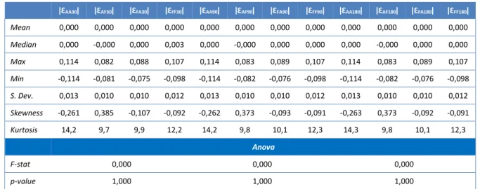
Table 2 presents descriptive statistics for the outcome of the measures of volatility estimated from the data of the PSI-20 and the application of equation (5) (ƐAAǀ, ǀƐFAǀ, ǀƐAFǀ and
ǀƐFFǀ, for 30, 90 and 180 days). Based on statistical evidence, the null hypothesis of equality
of means cannot be rejected and we conclude, with 99% confidence, that the average of the waste series does not differ across groups ƐAAǀ, ǀƐFAǀ, ǀƐAFǀ and ǀƐFFǀ.
Table 2. Descriptive statistics of the absolut return residuals volatility estimate (PSI-20)
ǀƐAA30ǀ ǀƐAF30ǀ ǀƐFA30ǀ ǀƐFF30ǀ ǀƐAA90ǀ ǀƐAF90ǀ ǀƐFA90ǀ ǀƐFF90ǀ ǀƐAA180ǀ ǀƐAF180ǀ ǀƐFA180ǀ ǀƐFF180ǀ
Mean 0,000 0,000 0,000 0,000 0,000 0,000 0,000 0,000 0,000 0,000 0,000 0,000 Median 0,000 -0,000 0,000 0,003 0,000 -0,000 0,000 0,000 0,000 -0,000 0,000 0,000 Max 0,114 0,082 0,088 0,107 0,114 0,083 0,089 0,107 0,114 0,083 0,089 0,107 Min -0,114 -0,081 -0,075 -0,098 -0,114 -0,082 -0,076 -0,098 -0,114 -0,082 -0,076 -0,098 S. Dev. 0,013 0,010 0,010 0,012 0,013 0,010 0,010 0,012 0,013 0,010 0,010 0,012 Skewness -0,261 0,385 -0,107 -0,092 -0,262 0,373 -0,093 -0,091 -0,263 0,373 -0,092 -0,091 Kurtosis 14,2 9,7 9,9 12,2 14,2 9,8 10,1 12,3 14,3 9,8 10,1 12,3 Anova F-stat 0,000 0,000 0,000 p-value 1,000 1,000 1,000
The calculated series using the opening prices of the day t and the day t+1 (ǀƐAA30ǀ,
ǀƐAA90ǀ, ǀƐAA180ǀ) present the greatest volatility (standard deviation of 0.0133) and the most
extreme maximum and minimum values (the maximum value is registered in the series ǀƐAA90ǀ and the minimum in the series ƐAA90ǀ and ǀƐAA180ǀ).
Only the series calculated using the opening and closing rates of a given day t (ǀƐAF30ǀ,
ǀƐAF90ǀ, ǀƐAF180ǀ) present positive skewness, which shows a trend for obtaining gain on the
same day, given that the positive distribution tail is longer. The remaining series record negative skewness, which may indicate a greater risk of substantial losses than gains of the same magnitude.
In turn, the excess of positive kurtosis found in all the series, is an indication of high market volatility, given the existence of peaks or stretching when compared to the normal distribution.
12
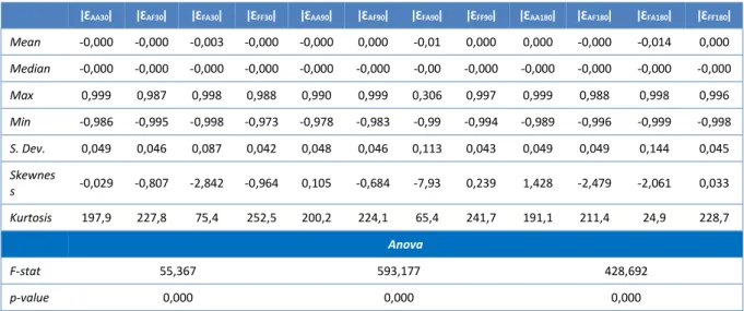
Similar tests were also applied to the data of the shares underlying the market index. Table 3 records the descriptive statistics of volatility measures estimated from the data of the shares underlying the market index (ǀƐAAǀ, ǀƐFAǀ, ǀƐAFǀ and ǀƐFFǀ, for 30, 90 and 180 days).
Table 3. Descriptive statistics of the absolute return residuals volatility estimate (shares underlying the market index)
ǀƐAA30ǀ ǀƐAF30ǀ ǀƐFA30ǀ ǀƐFF30ǀ ǀƐAA90ǀ ǀƐAF90ǀ ǀƐFA90ǀ ǀƐFF90ǀ ǀƐAA180ǀ ǀƐAF180ǀ ǀƐFA180ǀ ǀƐFF180ǀ
Mean -0,000 -0,000 -0,003 -0,000 -0,000 0,000 -0,01 0,000 0,000 -0,000 -0,014 0,000 Median -0,000 -0,000 -0,000 -0,000 -0,000 -0,000 -0,00 -0,000 -0,000 -0,000 -0,000 -0,000 Max 0,999 0,987 0,998 0,988 0,990 0,999 0,306 0,997 0,999 0,988 0,998 0,996 Min -0,986 -0,995 -0,998 -0,973 -0,978 -0,983 -0,99 -0,994 -0,989 -0,996 -0,999 -0,998 S. Dev. 0,049 0,046 0,087 0,042 0,048 0,046 0,113 0,043 0,049 0,049 0,144 0,045 Skewnes s -0,029 -0,807 -2,842 -0,964 0,105 -0,684 -7,93 0,239 1,428 -2,479 -2,061 0,033 Kurtosis 197,9 227,8 75,4 252,5 200,2 224,1 65,4 241,7 191,1 211,4 24,9 228,7 Anova F-stat 55,367 593,177 428,692 p-value 0,000 0,000 0,000
Contrary to the expected, the results obtained significantly differ from the ones using the PSI-20 data, as can be seen in Table 2. Indeed, it is possible to reject the null hypothesis of equality of means, and it can be concluded, with a confidence level of 99%, that the average of the waste series differs across groups ǀƐAAǀ, ǀƐFAǀ, ǀƐAFǀ and ǀƐFFǀ.
The AF series, calculated using the closing price of day t and the opening price of day t+1, are the more volatile, particularly when applied to the performance of the past 180 days – the series ǀƐFA180ǀ has a standard deviation of 0.1445. However, the maximum occurs
in the series ǀƐAA30ǀ with a value of 0.9997. It should be noted that with the exception of
series ǀƐFA90ǀi, in other series the maximum values recorded are very close to each other,
ranging between 0.9871 and 0.9996.In regards to the minimum value, there is also no remarkable variation between the series, and the minimum value is recorded in the series calculated using closing the price of day t and the opening price of the next day (t+1) applied to the profitability of the past 90 days (ǀƐFA90ǀ) at -0.9998. This series is one of the most
volatile, with a standard deviation of 0.1103.
As for skewness, only the series calculated using the opening prices of day t and t+1 (ǀƐAA90ǀ, ǀƐAA180ǀ) and the series calculated using the closing prices of day t and t-1 (ǀƐFF90ǀ e
ǀƐFF180ǀ), both applied to the performance of the past 90 and 180 days, show a higher
probability for gains than losses. Skewness in the other series is negative, and therefore there is occasion for potential loss.
Finally, the high kurtosis recorded in all series demonstrates that the shares underlying the PSI-20 show a high variation when compared to the mean.
In conclusion, it can be noted that the results obtained with PSI-20 and the shares underlying the market index differ amongst each other, in particular with regard to the series with the greatest prospect of gain. On the other hand, the excess of positive kurtosis recorded in all series, both of PSI-20 or shares underlying the market index, constitutes an indicator of high market volatility, which points to a destabilization in asset prices. The herding behaviour, the positive-feedback trading and market activity itself, measured by turnover, are just some of the factors that the financial literature points as causes of the increase in volatility.
13
4.2.2. Historical volatility
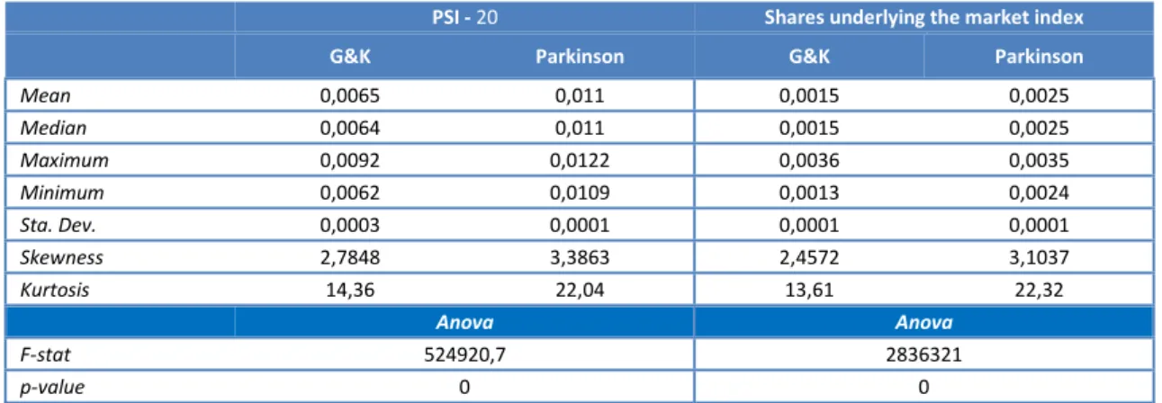
Table 4 summarizes the main descriptive statistics for the measures of historical volatility – Parkinson (1980) and Garman and Klass (1988) – calculated from PSI-20 data and from the shares underlying the market index.
Table 4. Descriptive statistics of the historical volatility:PSI-20 and shares underlying the market index
PSI - 20 Shares underlying the market index G&K Parkinson G&K Parkinson
Mean 0,0065 0,011 0,0015 0,0025 Median 0,0064 0,011 0,0015 0,0025 Maximum 0,0092 0,0122 0,0036 0,0035 Minimum 0,0062 0,0109 0,0013 0,0024 Sta. Dev. 0,0003 0,0001 0,0001 0,0001 Skewness 2,7848 3,3863 2,4572 3,1037 Kurtosis 14,36 22,04 13,61 22,32 Anova Anova F-stat 524920,7 2836321 p-value 0 0
The interpretation of the results allows us to infer that there are no significant differences between the estimated volatility measures, although Parkinson presents higher maximum and minimum values than Garman and Klass. However, Parkinson displays a lower variability (standard deviation) than Garman and Klass.
Regarding the skewness, values are significantly higher than in any of the series of absolute return residuals. The fact that the skewness shows positive values may indicate the achievement of gain, while excess kurtosis seems to show high market volatility.
Additionally, equations (6) and (7) were adapted to the data of the shares underlying the market index. Similar tests were applied, and the results reveal themselves to be identical to the PSI-20, as can be seen in Table 4.
Comparing the measures of historical volatility, it should be noted that Parkinson continues to present a higher minimum value but records a lower maximum value and a standard deviation identical to that of Garman and Klass. The excess kurtosis and (positive) skewness also seem to indicate high and asymmetric market volatility, with a higher probability for gains than losses of the same value. Subsequently, we calculated the correlation between the estimates of absolute return residuals and historical volatility – Parkinson (1980) and Garman and Klass (1988).
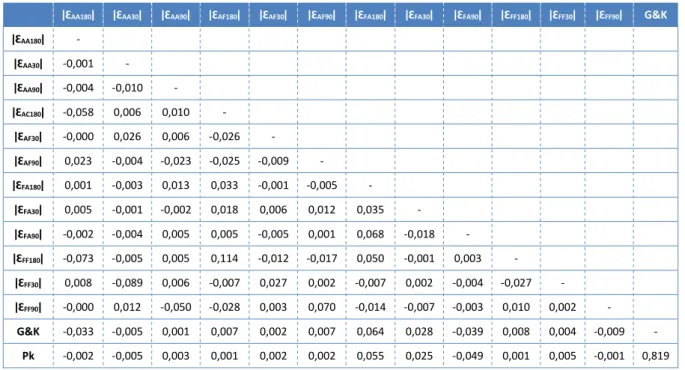
Tables 5 and 6 show the results of the correlation between the different volatility estimates for the data from PSI-20 and the shares underlying the market index, respectively.
As can be perceived, the correlation is relatively low, hence the use of different volatility estimates, each of them allowing us to obtain additional information. Parkinson (1980) and Garman and Klass (1988) volatility measures are those with a higher correlation value (0.813 with data from PSI-20 and 0.819 with data from the shares underlying the index), which is not in any way a surprising result given the inputs used for the calculation thereof.
14
Table 5. Analysis of the correlation between the different volatility estimates (PSI-20)
ǀƐAA180ǀ ǀƐAF90ǀ ǀƐAA30ǀ ǀƐAA90ǀ ǀƐAF180ǀ ǀƐAF30ǀ ǀƐFA180ǀ ǀƐFA30ǀ ǀƐFA90ǀ ǀƐFF180ǀ ǀƐFF30ǀ ǀƐFF90ǀ G&K
ǀƐAA180ǀ - ǀƐAF90ǀ 0,019 - ǀƐAA30ǀ 0,395 0,017 - ǀƐAA90ǀ 0,599 0,000 0,199 - ǀƐAF180ǀ -0,020 0,431 -0,019 0,000 - ǀƐAF30ǀ -0,058 -0,050 -0,056 0,000 -0,011 - ǀƐFA180ǀ 0,000 0,070 0,000 0,000 0,300 0,014 - ǀƐFA30ǀ 0,000 -0,058 -0,000 0,000 -0,141 0,241 0,026 - ǀƐFA90ǀ 0,008 0,252 0,008 0,000 0,081 0,030 0,527 0,052 - ǀƐFF180ǀ 0,000 -0,029 -0,000 0,000 -0,015 0,006 0,000 -0,001 0,001 - ǀƐFF30ǀ 0,000 -0,043 0,000 0,000 -0,024 -0,005 0,000 0,000 0,000 0,101 - ǀƐFF90ǀ 0,000 -0,000 -0,000 0,000 -0,001 0,053 0,000 -0,001 0,000 0,159 0,221 - G&K 0,010 -0,007 -0,005 0,018 -0,003 -0,003 -0,001 -0,009 0,003 - -0,009 0,001 -0,011 - Pk 0,003 -0,011 -0,000 0,022 -0,005 -0,005 -0,001 -0,001 0,003 - -0,001 0,001 0,002 0,813
Table 6. Analysis of the correlation between the different volatility estimates (shares underlying the market index)
ǀƐAA180ǀ ǀƐAA30ǀ ǀƐAA90ǀ ǀƐAF180ǀ ǀƐAF30ǀ ǀƐAF90ǀ ǀƐFA180ǀ ǀƐFA30ǀ ǀƐFA90ǀ ǀƐFF180ǀ ǀƐFF30ǀ ǀƐFF90ǀ G&K
ǀƐAA180ǀ - ǀƐAA30ǀ -0,001 - ǀƐAA90ǀ -0,004 -0,010 - ǀƐAC180ǀ -0,058 0,006 0,010 - ǀƐAF30ǀ -0,000 0,026 0,006 -0,026 - ǀƐAF90ǀ 0,023 -0,004 -0,023 -0,025 -0,009 - ǀƐFA180ǀ 0,001 -0,003 0,013 0,033 -0,001 -0,005 - ǀƐFA30ǀ 0,005 -0,001 -0,002 0,018 0,006 0,012 0,035 - ǀƐFA90ǀ -0,002 -0,004 0,005 0,005 -0,005 0,001 0,068 -0,018 - ǀƐFF180ǀ -0,073 -0,005 0,005 0,114 -0,012 -0,017 0,050 -0,001 0,003 - ǀƐFF30ǀ 0,008 -0,089 0,006 -0,007 0,027 0,002 -0,007 0,002 -0,004 -0,027 - ǀƐFF90ǀ -0,000 0,012 -0,050 -0,028 0,003 0,070 -0,014 -0,007 -0,003 0,010 0,002 - G&K -0,033 -0,005 0,001 0,007 0,002 0,007 0,064 0,028 -0,039 0,008 0,004 -0,009 - Pk -0,002 -0,005 0,003 0,001 0,002 0,002 0,055 0,025 -0,049 0,001 0,005 -0,001 0,819
In short, we realize that the results obtained confirm the presence of high volatility (asymmetric) in the Portuguese capital market, between July 1998 and June 2010, with a higher probability for gains than for losses of the same magnitude.
15
4.2.3. Obtaining series “clean” from the effects of the turnover and the day of the week
A common element taken into account by the different theories that analyze the impact of transactions of high volume of assets on the prices is that market activity is largely correlated with price variability – It takes volume to make prices move.
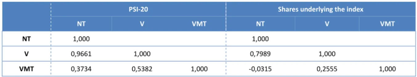
Table 7 provides results of the analysis of the correlation between the different measures of volume – volume of transactions in euro (V), number of transactions (NT) and average value of transactions in euros (VMT) – for the PSI-20 data and the data of the shares underlying the market indexii, respectively.
Table 7. Analysis of the correlation between the different volume measurements
PSI-20 Shares underlying the index
NT V VMT NT V VMT
NT 1,000 1,000
V 0,9661 1,000 0,7989 1,000
VMT 0,3734 0,5382 1,000 -0,0315 0,2555 1,000
Note: V - volume of transactions in euro, NT - number of transactions; VMT - average value of transactions in euros.
Regarding Table 7, it appears that in both cases the level of correlation is higher between the volume of transactions in euro and the number of transactions (0.9661 for PSI-20 and 0.7989 for the shares underlying the index) and that the remaining correlations are relatively low. We highlight a negative correlation between the average transaction value and number of transactions when volume measures are applied to the data of the shares underlying the market index. In fact, the value of the correlations between different measures of volume is lower when one considers the shares underlying the market index. This difference may possibly be due to the sheer size of the sample, because when the analysis focuses on the PSI-20, the series has about 3.500 observations in contrast to about 65.000 when the database corresponds to the shares underlying the market index.
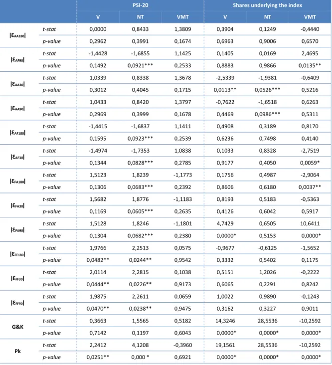
According to the procedure described in section 3.3.2, one obtains the results of the regressions estimated using the PSI-20 data from equations (8), (9) and (10), as shown in Table 8.
For the volume, measured using the average value of the transactions, one cannot reject the null hypothesis from the parameters. Indeed, the results show that, when explaining volatility, none of the parameters is statistically significant when compared to the estimates found at a significance level of 10%.
When the independent variable is the volume of transactions in euro, there seems to be a positive influence on volatility estimates calculated using the closing prices of day t and t-1 (ǀƐFF30ǀ, ǀƐFF90ǀ e ǀƐFF180ǀ) as well as in the volatility calculated using Parkinson's method.
Finally, the results indicate a positive influence of the number of transactions when explaining many of the volatility estimates, except for the one calculated using the opening prices of day t and t+1 (ǀƐAA30ǀ, ǀƐAA90ǀ, ǀƐAA180ǀ) and Garman and Klass‘s method. These results
seem consistent with the current theory that asserts the existence of a direct relationship between trading volume and market volatility. In fact, the volume measured by the number of transactions seems to explain market volatility, which may be due to, first, the large-block transactions undertaken or, quite simply, a large number of small investors, probably speculators, whose actions provide the necessary liquidity to capital markets, despite the fact that they generate volatility.
16
Table 8. Results of volume measurements
PSI-20 Shares underlying the index
V NT VMT V NT VMT ǀƐAA180ǀ t-stat 0,0000 0,8433 1,3809 0,3904 0,1249 -0,4440 p-value 0,2962 0,3991 0,1674 0,6963 0,9006 0,6570 ǀƐAF90ǀ t-stat -1,4428 -1,6855 1,1425 0,1405 0,0169 2,4695 p-value 0,1492 0,0921*** 0,2533 0,8883 0,9866 0,0135** ǀƐAA30ǀ t-stat 1,0339 0,8338 1,3678 -2,5339 -1,9381 -0,6409 p-value 0,3012 0,4045 0,1715 0,0113** 0,0526*** 0,5216 ǀƐAA90ǀ t-stat 1,0433 0,8420 1,3797 -0,7622 -1,6518 0,6263 p-value 0,2969 0,3999 0,1678 0,4469 0,0986*** 0,5311 ǀƐAF180ǀ t-stat -1,4415 -1,6837 1,1411 0,4908 0,3189 0,8170 p-value 0,1595 0,0923*** 0,2539 0,6236 0,7498 0,4140 ǀƐAF30ǀ t-stat -1,4974 -1,7353 1,0838 0,1033 0,8328 -2,7519 p-value 0,1344 0,0828*** 0,2785 0,9177 0,4050 0,0059* ǀƐFA180ǀ t-stat 1,5123 1,8239 -1,1773 0,1756 0,4987 -2,9064 p-value 0,1306 0,0683*** 0,2392 0,8606 0,6180 0,0037** ǀƐFA30ǀ t-stat 1,5682 1,8776 -1,1183 0,8193 0,5183 -0,5363 p-value 0,1169 0,0605*** 0,2635 0,4126 0,6042 0,5917 ǀƐFA90ǀ t-stat 1,5128 1,8246 -1,1801 4,7429 0,6505 10,6411 p-value 0,1304 0,0682*** 0,2380 0,0000* 0,5153 0,0000* ǀƐFF180ǀ t-stat 1,9766 2,2513 0,0575 -0,9677 -0,6125 -1,5652 p-value 0,0482** 0,0244** 0,9542 0,3332 0,5402 0,1175 ǀƐFF30ǀ t-stat 2,0114 2,2815 0,1038 0,5151 1,2026 -0,2222 p-value 0,0444** 0,0226** 0,9173 0,6065 0,2291 0,8242 ǀƐFF90ǀ t-stat 1,9875 2,2611 0,0659 1,0022 0,9890 -0,1243 p-value 0,0470** 0,0238** 0,9475 0,3162 0,3227 0,9011 G&K t-stat 0,3663 1,5565 0,5182 14,3246 28,5536 -10,2592 p-value 0,7142 0,1197 0,6043 0,0000* 0,0000* 0,0000* Pk t-stat 2,2412 4,1208 -0,3960 19,1561 28,5536 -10,2592 p-value 0,0251** 0,000 * 0,6921 0,0000* 0,0000* 0,0000*
* Significant at 1% level ** Significant at 5% level; *** Significant at 10% level
Note: V - volume of transactions in euro; NT - number of transactions; VMT - average value of transactions in euro
The major difference found in the results of the regressions applied to shares underlying the index, is that any of the volume measures considered – volume of euro transactions, number of transactions and average value of transactions in euro – have a positive influence on historical volatility, calculated using the Parkinson (1980) and Garman and Klass (1988) measures.
Furthermore, the average value of the transactions in euro can explain the volatility estimates ǀƐAA90ǀ, ǀƐAF30ǀ, ǀƐAF180ǀ and ǀƐFA90ǀ beyond the measures of historical volatility – note
that when considering the PSI-20, the results did not allow us to assess any causality relationship between the average value of the transaction and any of the volatility estimates considered.
17
Next we test the residuals, in order to check if any of the assumptions of the model is violated. The following conclusions are summarized below:
(i) the statistical results of the Bera and Jarque test, under the null hypothesis that the regression residues are normally distributed, show that the assumption of normalcy is not violated;
(ii) the statistical evidence for the null hypothesis of equal variances (Bartlett's test, Levene's test and Brown-Forsythe test) allow us to conclude with 95% confidence, that the null hypothesis cannot be rejected for any of the tests. In this sense, the assumption of homoscedasticity is not violated;
(iii) the results of the Ljung-Box Q-statistic for the null hypothesis of no autocorrelation in the residuals proposes, with 95% confidence, that the null hypothesis is not rejected.
Given the above, the option was to dispense with additional model adjustment testing, including nonparametric tests. The results, considering both the PSI-20 and the shares underlying the market index, are consistent with studies that positively relate volatility to the volume of transactions in the market, which somehow contradicts the very theory of market efficiency. Indeed, the market efficiency hypothesis maintains that price variability is not explained by turnover, with the demand curve of a title being (approximately) horizontal. In essence, this means that investors can buy or sell any amount of an asset without significantly affecting its market price.
4.2.4. The effect of herding on volatility
Table 9 shows the results of the regression estimated from equations (8), (9) and (10), which measure the effect of the herding intensity in daily volatility. The estimation of historical volatility is adjusted, “cleaned”, for the number of transactions, the volume of transactions in euro and the average of transactions in euro.
From the results obtained, we highlight the fact that the intensity of herding in neutral sequences (Hn), "clean" of the volume effect – the number of transactions, volume of transactions in euro and average value of transactions in euro – can explain the historical volatility estimated using Parkinson's measurement.
Note also that the intensity of herding in sequences of high, low and neutral, "clean" of the effect of volume of transactions in euro tends to explain the estimated volatility of the series calculated using closing prices and the profitability of 30 days (ǀƐFF30ǀ).
No additional model adjustment tests were performed because no violation of assumptions was detected. Indeed, the residues are normally distributed; the hypothesis of homoscedasticity and the absence of autocorrelation in the residuals are not rejected.
In short, in the situations identified above, the intensity of herding in the Portuguese capital market during the period of analysis explains its volatility. Thus, the results are consistent with the extensive financial literature that views herding as one of the factors that can destabilize the market [e.g., Banerjee (1992), Bikhchandani et al. (1992), Avramov et al. (2006)]. In other situations analyzed, we could not find statistical evidence that supports that herding positively influences market volatility.
18
Table 9. Results of herding in volatility estimates (PSI-20)
Ha Hb Υ Hn Ha Hb Η Hn Ha Hb Τ Hn ǀƐAA180ǀ t-stat -1,0746 -0,7588 -0,2350 -1,4730 -1,0532 0,4143 -1,4831 -1,1607 -1,2249 p-value 0,2826 0,4480 0,8142 0,1409 0,2924 0,6787 0,1381 0,2459 0,2207 ǀƐAA30ǀ t-stat -0,0868 -0,0699 -0,2757 1,0546 0,7812 0,4971 -0,5336 -0,4623 -1,0746 p-value 0,9308 0,9443 0,7828 0,2917 0,4347 0,6192 0,5936 0,6439 0,2618 ǀƐAA90ǀ t-stat -1,6291 -1,1730 -1,0772 -1,0212 -0,7594 -0,5337 -0,7377 -0,5466 -0,3742 p-value 0,1034 0,2409 0,2815 0,3073 0,4477 0,5936 0,4607 0,5847 0,7083 ǀƐAF180ǀ t-stat 0,4139 0,2622 0,0683 0,3741 0,1889 -0,0293 0,6748 0,5265 -0,2062 p-value 0,6790 0,7932 0,9455 0,7084 0,8502 0,9766 0,4998 0,5986 0,8367 ǀƐAF30ǀ t-stat -0,0868 -0,0699 -0,2757 0,1055 0,7812 0,4971 -0,5336 -0,4623 -1,0746 p-value 0,9308 0,9443 0,7828 0,2917 0,4347 0,6192 0,5936 0,6439 0,2826 ǀƐAF90ǀ t-stat 0,7639 0,4901 1,9305 0,4000 0,2723 -0,8709 0,6831 0,5152 -0,2096 p-value 0,4450 0,6241 0,0536 0,6892 0,7854 0,3839 0,4946 0,6065 0,8340 ǀƐFA180ǀ t-stat -0,5094 -0,4633 -1,9590 -0,4064 -0,3218 -2,0761 -0,6958 -0,5557 -0,5571 p-value 0,6105 0,6432 0,0502*** 0,6845 0,7477 0,0380 0,4866 0,5785 0,5775 ǀƐFA30ǀ t-stat 1,3985 1,1092 1,2776 0,1348 0,1069 -0,1267 1,0909 0,7976 -0,1393 p-value 0,1621 0,2675 0,2015 0,8928 0,9149 0,8992 0,2754 0,4251 0,8892 ǀƐFA90ǀ t-stat 0,2914 0,2036 -0,9908 -0,6702 -0,4940 0,5452 -0,2835 -0,2183 -0,3823 p-value 0,7708 0,8387 0,3218 0,5028 0,6213 0,5956 0,7768 0,8272 0,7023 ǀƐFF180ǀ t-stat -0,3329 -0,2488 -0,2090 0,0269 0,0537 1,1132 0,2755 0,2014 -0,2324 p-value 0,7392 0,8035 0,8345 0,9786 0,9572 0,2657 0,7829 0,8404 0,8162 ǀƐFF30ǀ t-stat 2,4616 1,9133 1,9209 -1,1222 -0,8869 -0,9925 -1,2590 -0,9926 0,2676 p-value 0,0139** 0,0558*** 0,0548*** 0,2618 0,3752 0,3211 0,2081 0,3210 0,7890 ǀƐFF90ǀ t-stat 0,0023 -0,0007 -0,0226 0,6814 0,5589 0,7810 1,0063 0,7334 0,0281 p-value 0,9982 0,9994 0,9820 0,4957 0,5763 0,4349 0,3144 0,4633 0,9776 G&K t-stat -0,6526 -0,7797 0,5975 -0,6253 -0,8958 1,0985 -1,2565 -1,1875 0,3182 p-value 0,5140 0,4356 0,5502 0,5318 0,3867 0,2721 0,2090 0,2351 0,7504 Pk t-stat 0,3428 0,4692 2,7478 -0,1324 -0,1779 2,2493 0,2167 0,3530 2,3996 p-value 0,7318 0,6390 0,006* 0,8947 0,8588 0,0246** 0,8284 0,7241 0,0165**
* Significant at 1% level ** Significant at 5% level; *** Significant at 10% level , , : dependent variables of the equations (8), (9) and (10)
4.3. Relationship between herding and profitability
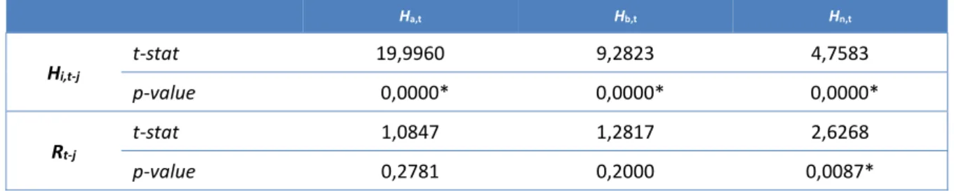
Examining the relationship between profitability and herding, estimated through the regression in accordance with equation (11), we obtained the statistics presented in Table 10.
Table 10. Results of the regression between herding and profitability (PSI-20)
Ha,t Hb,t Hn,t Hi,t-j t-stat 19,9960 9,2823 4,7583 p-value 0,0000* 0,0000* 0,0000* Rt-j t-stat 1,0847 1,2817 2,6268 p-value 0,2781 0,2000 0,0087* * Significant at 1% level
Our estimates lead us to the conclusion (with 99% confidence) that the intensity of herding in the current period is explained by the intensity of herding during the previous period. Moreover, the statistical results show that profitability is only statistically significant (with a level of significance of 1%) when explaining the intensity of herding in neutral sequences (Hn), characterized by price stability.
19
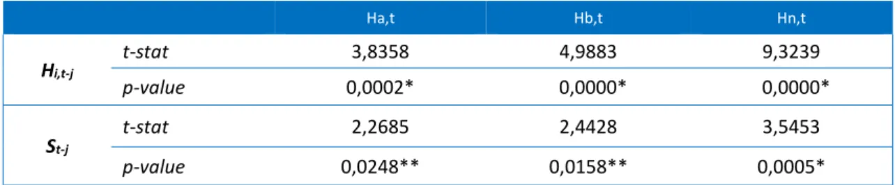
Thus, we conclude that the profitability of the index positively influences the intensity of herding in neutral sequences. Interestingly, the profitability of the index cannot explain the remaining sequences of herding, initiated by the buyer or by the seller and which, therefore, are characterized by prices variation. Finally, Table 11 summarizes the results of the estimated regression between profitability and intensity of herding, according to equation (12).
Table 11. Results of the regression between intensity of herding and profitability (PSI-20)
Ha,t Hb,t Hn,t Hi,t-j t-stat 3,8358 4,9883 9,3239 p-value 0,0002* 0,0000* 0,0000* St-j t-stat 2,2685 2,4428 3,5453 p-value 0,0248** 0,0158** 0,0005*
* Significant at 1% level; ** Significant at 5% level
The results indicate that none of the parameters is statistically significant and, therefore, that herding produces no change in profitability. This conclusion reinforces the previous results, where only a positive influence was found between herding and Parkinson’s historical volatility and between herding and volatility calculated using closing prices (applied to the profitability of the last 30 days).
5. Conclusion
The behavioural approach to finances has considerably contributed to explain the mechanisms of the capital markets. Admitting that investors’ behaviour may have a direct impact in the price of assets, influencing market volatility, constitutes a “giant step forward” in the field of finance. In effect, from the market efficiency theory to behavioural sciences, a long way must be run.
Market micro-structure is one of the most fascinating areas of finance, and many studies have been dedicated to pointing out the weaknesses of the market efficiency hypothesis. Despite the undeniable contribution of this theory, the truth is that some of the criticisms are easily understandable.
It is common sense that profit opportunities are there for "first hand" holders of information, tending to disappear as it spreads in the market and it is incorporated into asset prices. If everyone has access to the same information at the same moment in time, as suggested by the market efficiency theory, opportunities for profit will be minimal, if not non-existent. In addition, there is the fact that the majority of investors are rational which means that when confronted with the same information, they make identical investment decisions, considered to be the best among all possible. As a result, one can ask whether herding behaviour is a consequence of the rationality of investors. This is not the same as the market efficiency theory, which considers phenomena such as herding behaviour, feedback trading and noise-trading to be trading market anomalies.
To treat these phenomena as mere anomalies is to deny the evidence that (un)fortunately the Portuguese capital market has insisted on demonstrating, today, more than ever, the Portuguese financial market is suffering the effects of investors' expectations. The emotions of market participants, the (mis)information, the noise and the speculation are just some of the factors that contribute significantly to the process of price formation.
The present study has sought to analyse the behaviour of investors, particularly through the study of herding behaviour and its relationship with volatility and profitability.
20
A first conclusion refers that results demonstrate in regard to the shares included in the market index, traders tend to systematically mimic each other, consistent with, for example, the results obtained by Blasco et al. (2009). Indeed it is apparent, the predominance of high levels of herding in the transaction of shares underlying the PSI-20, particularly in sequences initiated by the buyer or the seller, when a price variation is registered.
Once the sample included shares underlying the market index and thus considered (at least from a theoretical standpoint) glamour stocks, the results appear consistent with authors like Black (1976), Froot et al. (1992) and Hirshleifer et al. (1994) who refer investors’ preference for this type of share against value stocks. Moreover, the results are still in line with authors such as Farrar and Girton (1981) and Del Guercio (1996) who reported that investors adjust their portfolios to the market index and prefer shares of bigger companies to those of neglected firms., although literature reveals that the latter have higher profitability.
A second conclusion to be drawn from this investigation relates to the volatility estimates – absolute return residuals and historical volatility. Results confirm that from July 1998 to June 2010, the Portuguese capital market showed levels of high and asymmetrical volatility, with greater probability for gain than for loss of the same magnitude.
On the other hand, the results of the regression estimates for this purpose, are in accordance with authors as Schwert (1989), Gallant et al. (1992) or Daigler and Wiley (1999), who positively relate market volatility to the volume of assets traded in capital markets. That conclusion opposes the market efficiency hypothesis, particularly because this theory believes that the demand curve of a title is (approximately) horizontal, and thus investors can buy or sell any amount of an asset without its price is significantly affected.
The existence of herding and a high (and asymmetrical) volatility in the capital market during the period is undeniable. In spite of this, the results are minimal when we attempt to determine the causal relationship between the intensity of herding and market volatility. Thus, the results obtained are consistent with authors such as Banerjee (1992), Bikhchandani et al. (1992) and Avramov et al. (2006), who propose herding as one cause for market volatility. In the present study, this relationship is established for the following situations: (i) in neutral sequences, the intensity of herding ("cleaned" of the effects of volume) explains the historical volatility estimated by the Parkinson measurement; (ii) in any one of the sequences considered (high, low or neutral), the intensity of herding ("cleaned" of the effect of trading volume in euro) positively influences the volatility calculated using closing prices (ǀƐFF30ǀ).
In the remaining situations, herding is not perceived to be an explaining factor for the volatility recorded in the Portuguese capital market between July 1998 and June 2010. These findings are further strengthened by the results of the statistical tests that confirm that herding produces no change in profitability.
In short, we can state that between July 1998 and June 2010, the Portuguese capital market recorded a high intensity of herding, which is more significant when there is price variation. Moreover, the market is volatile and asymmetric, with an increased probability for gain than for lossof the same magnitude. However, despite the existence of a positive relationship between herding and market volatility, the truth is that the results obtained are scarce in this sphere – intensity of herding can only explain historical volatility, estimated using the Parkinson measurement (1980), and volatility calculated using closing prices and profitability after 30 days. Statistical tests strengthen these results, confirming that intensity of herding has no impact on the profitability of the market index.
21
Alevy, J., Haigh, M., and List, J. 2003. Information cascades: evidence from a field experiment with financial market professional. Working Paper 03-15. Department of Agricultural and Resource Economics The University of Maryland, College Park
Avramov, D., Chordia, T., and Goyal, A. 2006. The impact of trades on daily volatility. The Review of Financial Studies 19 (4): 1241-1277.
Baker, M., and Wurgler, J. 2007. Investor Sentiment in the Stock Market. Journal of Economic Perspectives 21(2), 129-151
Baker, M., Wurgler, J., and Yuan, Y. 2012. Global, Local, and Contagious Investor Sentiment. Journal of Financial Economics 104(2): 272-287
Banerjee, A. 1992. A model of herd behaviour. Quarterly Journal of Economics 107: 797-817. Bhushan, R., Brown, D., and Mello, A. 1997. Do noise traders create their own space? Journal of Financial and Quantitative Analysis 32: 25-45.
Bikhchandani, S., and Sharma, S. 2000. Herd Behaviour in Financial Markets. IMF Staff Papers, 47(3), 279–310. Retrieved from http://www.jstor.org/stable/3867650
Bikhchandani, S., Hirshleifer, D. and Welch, I. 1992. A theory of fads, fashion, custom, and cultural change as informational cascades. Journal of Political Economy 100: 992-1096. Black, F. 1976. The dividend puzzle. Journal of Portfolio Management 2: 5-8.
Blasco, N., Corredor, C., Ferruela, G. 2009. The implications of herding on volatility. The case of the Spanish stock market. Working paper. Universidad Publica de Navarra. DT 98/09. Chan, K., and Fong, W. 2006. Realized volatility and transactions. Journal of Banking & Finance 30 (7): 2063-2085.
Chang, E., Cheng, J., and Khorana, A. 2000. An examination of herd behaviour in equity markets: an international perspective. Journal of Banking and Finance 24: 1651-1679. Daigler, R., and Wiley, M. (1999). The impact of trader type on the futures volatility – volume relation. Journal of Finance 52: 2297-2316.
Del Guercio, D. (1996). The distorcing effect of the prudent-man laws on institutional equity investments. Journal of Financial Economics 40: 31-62.
Devenow, A. and Welch, I. 1996. Rational herding in financial economics. European Economic Review 40, 603-615
Farrar, D., and Girton, L. 1981. Institutional investors and concentrations of financial power: berle and means revisited. Journal of Finance 36: 369-381.
Filip, A., Pece, A., Pochea, M. (2015). An Empirical Investigation of Herding Behaviour in CEE Stock Markets under the Global Financial Crisis, Procedia Economics and Finance 25: 354-361
Friedman, B. 1984. Discussion of Shiller. Brookings Papers on Economic Activity: 504-508. Froot, K., Scharfstein, D., Stein, J. 1992. Herd on the street: informational inefficiencies in a market with short-term speculation. Journal of Finance 47: 1461-1484.
Gallant, R., Rossi, P., and Tauchen, G. 1992. Stock priecs and volume. Review of Financial Studies 5: 199-242.
Garman, M., and Klass, M. 1988. On the estimation of security price volatilities from historical data. Journal of Business 53: 67-78.
Gompers, P. and Metrick, A. 2001. Institutional investors and equity prices. Quartely Journal of Economics 116: 229-260.
22
Henker, J., Henker, T., and Mitsios, A. 2006. Do investors herd intraday in the Australian equities? International Journal of Managerial Finance 2 (3): 196-219.
Hirshleifer, D. and Teoh, S. 2001. Herd Behaviour and Cascading in Capital Markets: A Review and Synthesis. Munich Personal RePEc Archive MPRA. Paper No. 5186, posted 7. October 2007 Online at http://mpra.ub.uni-muenchen.de/5186/
Hirshleifer, D., Subrahmanyam, A., Titman, S. 1994. Security analysis and trading patterns when some investors receive information before others. Journal of Finance 49: 1665-1698. Hwang, S., and Salmon, M. 2004. Market stress and herding. Journal of Empirical Finance 11: 585-616.
Jain, A., and Gupta, S. 1987. Some Evidence on "Herding" Behaviour of U. S. Banks. Journal of Money, Credit and Banking, 19(1), 78–89.
Lakonishok, J.; Shleifer, A.; Thaler, R., and Vishny, R.W. 1994. Contrarian investment, extrapolation, and risk. Journal of Finance 49: 1541-1478.
Lintner, G. (1998). Behavioural finance: Why investors make bad decisions. The Planner 13 (1): 7-8.
Lugo, S., Croce, A., and Faff, R. (2015). Herding Behaviour and Rating Convergence among Credit Rating Agencies: Evidence from the Subprime Crisis. Review of Finance, 19 (4):1703-1731.
Maug, E., and Naik, N. (2011). Herding and delegated portfolio management. The impact of relative performance evaluation on asset allocation. Quarterly Journal of Finance, 01:265 Parkinson, M. (1980). The random walk problem: extreme value method for estimating the variance of the displacement. Journal of Business 53: 61-65.
Patterson, D., and Sharma, V. (2010). The Incidence of Informational Cascades and the Behavior of Trade Interarrival Times During the Stock Market Bubble. Macroeconomic Dynamics 14 (Supplement 1): 111-136
Puckett, A., and Yan, X. (2008). The determinants and impact of short-term institutional herding. Working paper. Available at SSRN (http://ssrn.com/abstract=972254)
Rajan, R. (1994). Why credit policies fluctuate: a theory and some evidence. Quartely Journal of Economics 436: 399-442.
Roll, R. (1992). A mean/variance analysis of tracking error. Journal of Portfolio Management (Summer): 13-22.
Scharfstein, D., and Stein, J. (1990). Herd behaviour and investment. American Economic Review 80: 465-479.
Schwert, W. (1989). Why does stock market volatility change over time?. Journal of Finance 44: 1115-1153.
Sias, R. (2004). Institutional herding. Review of Financial Studies 17 (1): 165-206.
Tan, L., Chiang, C., Mason, J., and Nelling, E. (2008). Herding behaviour in Chinese stock markets: An examination of A and B shares. Pacific-Basin Finance Journal, 16 (1–2), p. 61-77 Trueman, B. (1994). Analyst forecasts and herding behaviour. Review of financial studies 7: 97-124.
Wermers, R. (1999). Mutual fund herding and the impact sock prices. Journal of Finance 54: 581-622.