Harvesting in a Random Varying Environment: Optimal, Stepwise and Sustainable Policies for the Gompertz Model

(1)

Published online in International Academic Press (www.IAPress.org)

Harvesting in a Random Varying Environment: Optimal, Stepwise and

Sustainable Policies for the Gompertz Model

Nuno M. Brites

1,∗

, Carlos A. Braumann

1,2

1_{Centro de Investigação em Matemática e Aplicações, Instituto de Investigação e Formação Avançada, Universidade de ´}_{Evora, Portugal} 2_{Departamento de Matemática, Escola de Ciências e Tecnologia, Universidade de ´}_{Evora, Portugal}

Abstract In a random environment, the growth of a population subjected to harvesting can be described by a stochastic differential equation. We consider a population with natural growth following a Gompertz model with harvesting proportional to population size and to the exerted fishing effort. The main goal of this work is to compare the performance of three fishing policies: one with variable effort, named optimal policy, the second based on variable effort but with small periods with constant effort, named stepwise policy, and another with constant effort, denoted by optimal sustainable policy. We will show that the first policy is inapplicable from the practical point of view, whereas the second one, although being suboptimal, is applicable but has some shortcomings common to the optimal policy. On the contrary, the constant effort policy is easily implemented and predicts the sustainability of the population as well as the existence of a stationary density for its size. The performance of the policies will be assessed by the profit obtained over a finite time horizon. We also show how changes in the parameter values affect the profit differences between the variable effort policy and the constant effort policy.

Keywords Stochastic Differential Equations, Stationary Density, Sustainable Effort, Stochastic Optimal Control, Constant Effort, Stepwise Policy, Gompertz Model.

AMS 2010 subject classifications60H10, 92D25, 93E20, 60H35 DOI:10.19139/soic-2310-5070-830

1. Introduction

Stochastic optimal control methods have been applied to obtain optimal harvesting policies in a randomly varying environment (see, for instance, [2], [3], [13] and [17]). To apply such policies, the fishing effort,E(t), must be adjusted at every time instant, according to the random variation of the population size. This will cause sudden and frequent transitions between maximum or high harvesting efforts and low or null harvesting efforts. Such transitions in effort are not compatible with the logistics of fisheries. Besides, periods of low or no harvesting pose social and economical undesirable implications (intermittent unemployment is just one of them). In addition to such shortcomings, to define the appropriate level of effort, the optimal policies require the knowledge of the population size at every time instant, which is a time consuming, inaccurate and expensive task. Therefore, the optimal policies with variable effort are inapplicable and should be considered unacceptable.

In [6] and [7], a constant fishing effort,E(t)≡ E, was assumed and, for a large class of models, it was found that there is, under mild conditions, a stochastic sustainable behaviour for the population size. Namely, the probability distribution of the population size at timetwill converge, ast→ +∞, to an equilibrium probability distribution (the so-called stationary or steady-state distribution) having a probability density function (the so-called stationary ∗_{Correspondence to: Nuno M. Brites (Email: brites@uevora.pt). Centro de Investigação em Matemática e Aplicações, Instituto de} Investigação e Formação Avançada, Universidade de Évora, Rua Romão Ramalho, 59, 7000-671, Évora, Portugal

(2)

density). In particular, for the Gompertz model, the stationary density was found, and the constant effort that optimizes the steady-state yield was determined. The issue of profit optimization, however, was not addressed.

In a previous work ([9]), we have developed, as an alternative to the variable effort policies, a sustainable constant effort policy based on profit optimization, which is extremely easy to implement and leads to a stochastic steady-state. We have determined the constant effort that maximizes the expected profit per unit time at the steady-state, in the general case and for the specific cases of the logistic (see also [10]) and the Gompertz models. One might think that a constant effort policy would result in a substantial profit reduction compared with the optimal variable effort policy, but we have shown, using realistic data from two harvested populations, that this is not the case. This new policy, rather than switching between large and small or null fishing effort, keeps a constant effort and is therefore compatible with the logistics of fisheries. Furthermore, this alternative policy does not require knowledge of the population size and it is very easy to implement.

Another alternative to the optimal variable effort policy is discussed in this paper. We present, for the Gompertz model, a sub-optimal policy, named stepwise policy, where the harvesting effort under the optimal variable effort policy is determined at the beginning of each year (or at the beginning of a larger period, for instance, two years) and kept constant during that year. This policy is not optimal and still poses some social problems, but has the advantage of being applicable, since the changes in effort are less frequent and compatible with the fishing activity. Furthermore, although we still need to keep estimating the fish stock size, we do not need to do it so often. Replacing the optimal variable effort policy by a stepwise policy has the advantage of applicability but, at best, considerably reduces the already small profit advantage of the optimal variable effort policy over the optimal constant effort policy. In some cases, the optimal sustainable policy even outperforms this stepwise policy in terms of profit.

This paper is organized as follows. In Section2, we develop the optimal variable effort policy. We also present in this section the stepwise policy. In Section 3, we obtain the optimal sustainable policy based on stochastic differential equations theory. Section4refers to the comparisons of the above policies and to the effect on the profit of changes in the parameter values. Finally, some concluding remarks are given in Section5.

2. Policies based on optimal control theory

Throughout this paper,X(t)represents the population size at the time instantt, and follows a Gompertz growth model. Population size can be measured in terms of biomass or numbers of individuals. We consider a stochastic framework, i.e. the population lives in a random environment and its (per capita) growth is affected by a random noise, which we approximate by a standard white noise (as in [2], [4], [8] and [16]). The harvesting rate,H(t), is formulated under the assumption (see [11]) that harvesting is proportional to the population size and to the exerted fishing effort, i.e.H(t) = qE(t)X(t). So, the population growth model under harvesting and in a randomly varying environment can be described by the Stochastic Differential Equation (SDE)

dX(t) = rX(t) ln ( K X(t) ) dt− qE(t)X(t)dt + σX(t)dW (t), X(0) = x, (1)

where r > 0 represents a growth rate parameter, K > 0 is the carrying capacity (deterministic environment equilibrium),q > 0 is the catchability coefficient, σ > 0 measures the random fluctuations intensity,W (t) is a standard Wiener process andx > 0is the initial population size.

Here, we follow [11] and assume that the price (or revenue) per unit of harvesting, p(H(t)), may decrease when the yieldH(t)(amount of fish harvested per unit time) increases. Thus, we choosep(H(t)) = p1− p2H(t), withp1> 0and p2≥ 0. The (total) price per unit time is thereforeP (t) = p(H(t))H(t) = (p1− p2H(t))H(t). An increase in effort implies an increase in the unit cost, since very high effort values will require the use of less efficient vessels and less adapted fishing technologies, for instance. Therefore, the cost per unit effort is represented byc(E(t)) = c1+ c2E(t), withc1≥ 0andc2> 0. The (total) cost per unit time is proportional to the cost per unit effort,C(t) = c(E(t))E(t). Finally, the profit per unit time,Π(t), is just the difference between revenues and costs, Π(t) = P (t)− C(t).

(3)

The optimal policy with variable effort consists in maximizing the profit over a finite time horizon, T > 0. However, the optimization process must take into account the following considerations:

• X(t)is a stochastic process, so the optimization will refer to the mean value ofX(t),E[X(t)], instead of the process itself.

• the effort is constrained to a minimum value and maximum value:0≤ Emin≤ E(t) ≤ Emax< +∞.

• profit values correspond to a currency amount, so currency depreciation, cost of opportunity losses and social rates are all integrated within a discount rateδ. Therefore, we will work with the present valuee−δtΠ(t).

• for a timet∈ [0, T ], we defineJ (y, t) :=E[∫_tTe−δ(τ−t)Π(τ )dτ|X(t) = y]as the expected discounted future profits when the population size at timetisy.

Summing up, the optimal policy with variable effort is in fact the solution of a stochastic optimal control problem (SOCP), in which, for a time period[0, T ], the goal is to maximize the expected accumulated discounted profit earned by the harvester (present value),

V∗:= J∗(x, 0) = max E(τ ) 0≤τ≤T E   T ∫ 0 e−δτΠ(τ )dτX(0) = x  , (2)

consideringE(t)the control andX(t)the state variable, subject to the growth dynamics given by (1) and to the terminal conditionJ∗(X(T ), T ) = 0. This SOCP is solved by applying dynamic programming (see [5], [9] and [12]), which in turn reduces to solve the Hamilton-Jacobi-Bellman (HJB) equation

−∂J∗(X(t), t) ∂t = Π ∗_(t)_{− δJ}∗_{(X(t), t) +}∂J∗(X(t), t) ∂X(t) ( r ln ( K X(t) ) − qE∗_(t))_X(t) + σ 2_X2_(t) 2 ∂2J∗(X(t), t) ∂X2_(t) , (3)

whereE∗(t)represents the constrained optimal variable effort. This is given by

E∗(t) =            0,( if E_{f ree}∗ (t) < Emin p1− ∂J∗(X(t),t) ∂X(t) ) qX(t)− c1 2 (p2q2X2(t) + c2)

, if Emin≤ Ef ree∗ (t)≤ Emax

Emax, if E_{f ree}∗ (t) > Emax,

whereE_{f ree}∗ (t)is the unconstrained effort (see [13] and [17]), andΠ∗(t) = Π(t)|E(t)=E∗(t).

Note that, to solve equation (3) numerically, we use a discretization scheme in time and space. Since it is a parabolic partial differential equation, the Crank-Nicolson discretization scheme is more suitable (see [9,10]). To apply the Crank-Nicolson scheme, time and space intervals should be partitioned into sub-intervals, ideally with a very small and close to zero amplitude. Here, the time interval [0, T ] was divided into n sub-intervals with∆t = T /nlength, and the space interval was restricted to[0, Xmax] and divided intomsub-intervals with

(4)

The approximations ∂J_i,j∗ ∂t ≈ J_i,j+1∗ − J_i,j∗ ∆t , ∂J_i,j∗ ∂x ≈ 1 2 ( J_i+1,j+1∗ − J_i∗_−1,j+1 2∆x + J_i+1,j∗ − J_i∗_−1,j 2∆x ) , ∂2_J∗ i,j ∂x2 ≈ 1 2 (J_i+1,j+1∗ −J_i,j+1∗ ∆x − J_i,j+1∗ −J_i−1,j+1∗ ∆x ∆x + J_i+1,j∗ −J_i,j∗ ∆x − J_i,j∗ −J_i−1,j∗ ∆x ∆x )

were used in the interior of(0, T )× (0, Xm), withJ_i,j∗ = J∗(Xi, tj). Approximations for the boundary points can be seen in [9].

2.1. Stepwise policy

To obtain the optimal variable effort policy we need to compute the optimal effort in each of the points of the above grid. Since we are dealing with a SOCP without any regularizing penalization (the inclusion of a regularizing penalization is treated in a forthcoming paper), one expects to have frequently and very abrupt changes on the effort, resulting in an inapplicable policy from the point of view of the fishing activity.

One way to mitigate this behaviour is to consider sub-optimal policies based on stepwise effort. We define a stepwise effort as the harvesting effort, determined under the optimal variable effort policy at the beginning of a time sub-interval with durationp(for instance, 1 or 2 years), and kept constant during that sub-interval. We use

p = v∆t(vis a positive integer) to be a multiple of the time step∆tused in the numerical computations and in the Monte Carlo simulations. So, in this stepwise effort policy, for timetin the period[lp, (l + 1)p[ = [tlv, t(l+1)v[, we keep the effortE_step∗ (t) = E∗(lp)constant and equal to the effort of the optimal policy at the beginning of the period.

This policy is obviously not optimal. Since it is a stepwise modification of the optimal variable effort policy, it is not even optimal among the stepwise policies. However, it is, as it should, non-anticipative, i.e. it does not use future values of the fish population size, which are unknown at the time of the decision. This will not eliminate the frequent and very abrupt effort changes, but will result in an applicable policy. In Section4we will show an application with stepwise effort.

(5)

3. Optimal sustainable policy based on stochastic differential equations theory

The optimal sustainable policy considers the application of a constant harvesting effort across time. For this policy, the population dynamics under Gompertz growth is given by

dX(t) = rX(t) ln ( K X(t) ) dt− qEX(t)dt + σX(t)dW (t), X(0) = x > 0. (4)

To solve this equation, we can apply the change of variableY (t) = ln X(t), and the Itˆo Theorem (see [16]) to obtain dY (t) = r (ln K− Y (t)) dt − ( qE +σ 2 2 ) dt + σdW (t). (5)

Equation (5) is a linear stochastic differential equation. So, we can multiply equation (5) by the integrating factor

ert_{and, after some algebra, obtain}

d(ertY (t))= ( r ln K− qE −σ 2 2 ) ertdt + σertdW (t).

Integrating this equation over the interval[0, t]and simplifying yields

Y (t) = Y (0)e−rt+ ( ln K−qE r − σ2 2r ) ( 1− e−rt ) + σe−rt t ∫ 0 ersdW (s). (6)

Finally, by transforming back toX(t)gives

X(t) = eY (t)= exp { e−rtln x } exp { ( ln K−qE r − σ2 2r ) ( 1− e−rt )} exp { σe−rt t ∫ 0 ersdW (s) } ,

which is the solution of equation (4). We notice that, in (6), the integrand of

t

∫ 0

ers_{dW (s)}_{is deterministic and so the stochastic integral is Gaussian}

with mean 0 and variance∫₀t(ers)2ds = _2r1 (e2rt− 1). Therefore,Y (t)is Gaussian with meanµ(t) = e−rtln x + ( ln K−qE_r −σ2 2r ) (1− e−rt)and varianceθ2_{(t) =} σ2 2r ( 1− e−2rt).

Whent→ +∞, the limit r. v.Y_∞has meanµ = ln K−qE_r −σ_2r2 and varianceθ2₌σ2

2r. From [7], the stationary density ofX_∞= eY_∞_is p(x) = 1 θ√2πxexp { −(ln x− µ)2 2θ2 } , 0 < x < +∞,

and the first and second moments of X_∞ are E[X_∞] = K exp { −qE r − σ2 4r } and E[X2 ∞] = K2exp { −2qE r } , respectively.

The steady-state structure of the profit per unit time is similar to the case of the optimal policy and is given by Π_∞= P_∞− C = (p1qX∞− c1)E− (p2q2X_∞2 + c2)E2,whereP∞is the sale price per unit time,Cis the fishing cost per unit time andH_∞:= qEX_∞is the sustainable harvesting rate. We define the expected sustainable profit per unit time as

E[Π_∞] = E[(p1qX∞− c1)E− (p2q2X_∞2 + c2)E2 ] = (p1qE[X∞]− c1)E− (p2q2E [ X_∞2]+ c2)E2 = ( p1qK exp { −qE r − σ2 4r } − c1 ) E− ( p2q2K2exp { −2qE r } + c2 ) E2.

(6)

The optimal sustainable policy with constant effort consists in maximizing the expected sustainable profit per unit time, i.e.

max E_≥0E[Π∞] = maxE_≥0 (( p1qK exp { −qE r − σ2 4r } − c1 ) E− ( p2q2K2exp { −2qE r } + c2 ) E2 ) ,

to obtain the optimal constant effort E∗∗ (satisfying dE[Π_∞]/dE = 0and d2_E_[Π

∞]/dE2< 0) and the optimal

expected sustainable profit E[Π∗∗_∞] = ( p1qK exp { −qE∗∗ r − σ2 4r } − c1 ) E∗∗− ( p2q2K2exp { −2qE∗∗ r } + c2 ) E∗∗2.

FromE∗∗one can also obtain the mean value of the population size under the optimal sustainable effort, E[X_∞∗∗] = K exp { −qE∗∗ r − σ2 4r } .

Contrary to the optimal variable effort policy, the optimal sustainable effort policy with constant effort is very easy to compute and to apply.

4. Comparison of the policies

The comparison, in terms of the expected accumulated discounted profit, of the optimal variable effort policy and the optimal sustainable constant effort policy cannot be done directly, since the first one maximizes the accumulated discounted profit over a finite time interval[0, T ]and the second one maximizes the profit per unit time asT → ∞. So, for comparisons purposes, we define:

• Π∗_{(t) = (p}₁_qX(t)_{− c}₁_)E∗_(t)_{− (p}₂_q2_X2_{(t) + c} 2)E∗

2

(t), the optimal profit per unit time under the optimal variable effortE∗(t);

• Π∗

step(t) = (p1qX(t)− c1)Estep∗ (t)− (p2q2X2(t) + c2)E∗ 2

step(t), the profit per unit time under the stepwise

variable effortE_step∗ (t);

• Π∗∗_{(t) = (p}₁_qX(t)_{− c}₁_)E∗∗_{− (p}₂_q2_X2_{(t) + c} 2)E∗∗

2

, the optimal sustainable profit per unit time under the optimal sustainable effortE∗∗.

The following expected accumulated discounted profits, for the 3 policies are: (A) V∗=E

[_∫_T 0

e−δτΠ∗(τ )dτX(0) = x

]

, the optimal present value under the optimal variable effortE∗(t).

(B) V_step∗ =E [_∫_T

0

e−δτΠ∗_step(τ )dτX(0) = x

]

, the optimal present value under the stepwise effortE_step∗ (t), kept constant on intervals of durationp.

(C) V∗∗=E [∫T

0

e−δτΠ∗∗(τ )dτX(0) = x

]

, the optimal present value under the optimal sustainable effortE∗∗. To compute these profits, we resort to Monte Carlo simulations, with an Euler scheme, from which we took 1000 sample paths for the population, effort and profit. We have used realistic biological and economic parameters (found in [14]) concerning the Bangladesh shrimp (Penaeus monodon), a species for which the Gompertz growth model

(7)

Item Description Value Unit

r Growth rate parameter 1.331 year−1

K Carrying capacity 11400 tonnes

q Catchability coefficient 9.77· 10−5 SFU−1year−1

Emin Maximum fishing effort 0 SFU

Emax Maximum fishing effort r/q SFU

σ Strength of environmental fluctuations 0.2 year−1/2

x Initial population size 0.5K tonnes

δ Discount factor 0.05 year−1

p1 Linear price parameter 8362.3 BDT·tonnes−1

p2 Quadratic price parameter 0 BDT·year·tonnes−2

c1 Linear cost parameter 1156.8 BDT·SFU−1year−1

c2 Quadratic cost parameter 10−2 BDT·SFU−2year−1

T Time horizon 50 year

n Number of time sub-intervals 300

∆t Amplitude of time sub-intervals 2 month

Xmax Maximum population level 2K tonnes

m Number of sub-intervals for the space state 150

∆x Amplitude of space state sub-intervals 152 tonnes

Table 1. Parameter values used in the simulations. The Standardized Fishing Unit (SFU) measure is defined in [14]. BDT stands for Bangladesh Taka. At January 1, 2011, the currency exchange rate was 1 BDT = 0.0106 Euros

(see https://www.exchangerates.org.uk/EUR-BDT-01_01_2011-exchange-rate-history.html,

accessed on July 23, 2018). We chooseXmax= 2Kin order to include practically all possible simulated values ofX(t).

seems to be more appropriate (see [1]). For some parameters there was no available information, namelyσ,δ,p2 andT. For those, we choose typical values (borrowed from similar studies (see [10])). Other parameters without information were set with realistic values, as in the case ofEmin,Emax andXmax. The full list of parameters

is shown in Table1, which also shows the values used for the application of the Crank- Nicolson discretization scheme.

Table2shows the present value profits (A), (B) and (C), i.e.V∗,V_step∗ and V∗∗, the corresponding standard deviations and the relative cross-differences among them. For the stepwise policy, we have chosen time sub-intervals with a duration ofp = 1year, i.e., the optimal effort is determined at the beginning of each year and kept constant during that year.

An overall conclusion from Table2is that the relative differences among profits are small. Since (A) refers to an optimal policy and (B) refers to a sub-optimal policy, it is not surprising that the relative difference (6.3%) between (A) and (B) is positive. It is however surprising to see that the profit advantage of the optimal policy with variable effort (A) over the optimal sustainable policy with constant effort (C) is only 1.5%. This raises a question that could be addressed to fishery managers: are you willing to ”loose“, on average, 1.5% of the hypothetical profit and maintain always the same number of vessels, the same number of gears, the same number of manpower hours (just

(8)

Policy Profit value Standard deviation Relative differences (%) (A) V∗= 594.14 21.40 V ∗_{− V}∗ step V∗ = +6.3 V∗− V∗∗ V∗ = +1.5 (B) V_step∗ = 556.61 24.29 V ∗ step− V∗ V_step∗ =−7.7 V_step∗ − V∗∗ V_step∗ =−5.1 (C) V∗∗= 585.00 21.11 V ∗∗_{− V}∗ V∗∗ =−1.5 V∗∗− V_step∗ V∗∗ = +4.8

Table 2. Numerical comparisons between the profit obtained by the application of the optimal policy (A), the policy with stepwise effort (B) and the sustainable optimal policy (C), and their relative cross differences. We also present the profit standard deviation. Profit values are in million BDT.

to give a few examples), instead of keep changing them abruptly at each time instant? It is our opinion that the answer to this question would be favourable to the new sustainable policy presented here.

The application of a stepwise policy (with 1-year steps) instead of the optimal sustainable policy will cause a reduction of 5.1%, on average. This reinforces, for the model and parameters used here, that the sustainable policy could indeed be the best option.

Regarding the standard deviation of the present value profit among the 1000 simulated trajectories, the values obtained for the three policies are quite similar, although slightly higher for the stepwise policy.

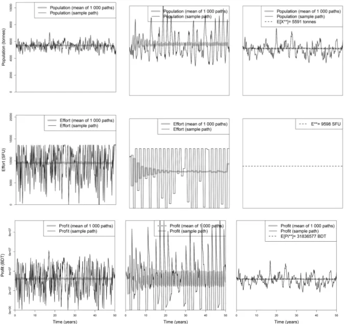
The black thin lines on Figure1show, for the three policies (A), (B) and (C), one path for the population, effort and profit per unit time, randomly chosen among the 1000 simulated sample paths. The thicker gray lines refer to the mean of the 1000 sample paths, and the black dashed lines presents the constant values from the sustainable policy given by the expressions at the end of Section 3.

The three policies behave quite differently. The stepwise policy presents huge variations in terms of the population size, which are accompanied by the also huge variations in effort and profit per unit time. The optimal policy exhibits frequent and abrupt changes on effort and profit per unit time, contrasting with the corresponding trajectories for the optimal sustainable policy, which shows a constant effort and a smaller magnitude oscillation in the profit per unit time.

The depicted trajectory is one of the possible outcomes that the harvester may experience. In terms of the population size, the optimal policy produces the trajectory with less size oscillations. Note that, for the policies with variable effort, harvesters should adjust the fishing effort at every time instant. Effort adjustments often correspond to changes from periods with zero effort (i.e., the fishery is closed) to periods with maximum effort (i.e., fishing with all available equipments and manpower). Clearly, this is not applicable since abrupt and frequent changes on effort are not compatible with the logistic of fisheries and, in addition, it is not feasible to obtain information on population size all the time. On the contrary, the optimal sustainable policy implies the application of a constant effort at every time instant, making this policy very easy to implement by harvesters. We foresee that such policy, if available to fishery managers, can be clearly desirable, even with the slight profit reduction of about 1.5%. Another possible policy, without the shortcomings of the optimal variable policy, is the stepwise policy. This one is suboptimal but has the advantage of being applicable. However, the problem of frequent and abrupt changes on effort still exists, although less frequently. Furthermore, this stepwise policy, being a stepwise non-anticipative modification of the optimal variable effort policy, can be less profitable than the optimal sustainable constant effort policy; this is indeed what happened in the case of this fishery (see Table2, comparison C).

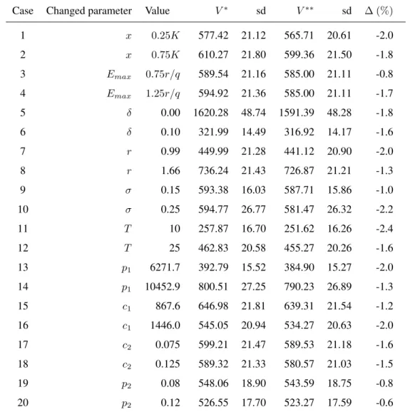
4.1. Alternative cases with parameters variations

One might think that the advantages of the optimal sustainable policy over the optimal variable effort policy depends on the parameters and model used. In a previous work [10], we have shown, for the logistic case, other profit structure and other population parameters (i.e., for a different species), that the reduction in profit is also quite small. Other conclusions related to the policies performance are similar to the ones presented here. Nevertheless, to evaluate the consequences of changes in the parameter values, we present now alternative cases (see Table

(9)

Figure 1. Mean and randomly chosen sample path for the population (first row), the effort (second row) and the profit per unit time (third row) for the three policies: optimal variable effort policy (first column), stepwise policy (second column) and optimal sustainable policy (third column).

3) that correspond to variations in the parameters shown in Table 1, usually 25% lower and 25% higher, with some exceptions that we now indicate. Since the initial population parameterxwas set as0.5K, we consider as alternatives the lower value0.25K(case 1) and the higher value0.75K(case 2). For theδparameter, we consider two alternative values, 0 and 0.10 (cases 5 and 6, respectively). SinceT is high, we consider two alternative lower valuesT = 10(case 11) andT = 25(case 12). Case 19 corresponds to a positivep2 value and case 20 considers an increase of50%inp2.

We also show on Table3the profit values (A) and (C), corresponding to the application of the optimal variable effort and optimal sustainable constant effort policies, and their relative profit differences.

A general comment concerning Table 3is that, for almost all the cases, the percent reduction of profit, ∆, incurred by using the optimal constant effort policy instead of the optimal variable effort policy is quite small,

(10)

Case Changed parameter Value V∗ sd V∗∗ sd ∆ (%) 1 x 0.25K 577.42 21.12 565.71 20.61 -2.0 2 x 0.75K 610.27 21.80 599.36 21.50 -1.8 3 Emax 0.75r/q 589.54 21.16 585.00 21.11 -0.8 4 Emax 1.25r/q 594.92 21.36 585.00 21.11 -1.7 5 δ 0.00 1620.28 48.74 1591.39 48.28 -1.8 6 δ 0.10 321.99 14.49 316.92 14.17 -1.6 7 r 0.99 449.99 21.28 441.12 20.90 -2.0 8 r 1.66 736.24 21.43 726.87 21.21 -1.3 9 σ 0.15 593.38 16.03 587.71 15.86 -1.0 10 σ 0.25 594.77 26.77 581.47 26.32 -2.2 11 T 10 257.87 16.70 251.62 16.26 -2.4 12 T 25 462.83 20.58 455.27 20.26 -1.6 13 p1 6271.7 392.79 15.52 384.90 15.27 -2.0 14 p1 10452.9 800.51 27.25 790.23 26.89 -1.3 15 c1 867.6 646.98 21.81 639.31 21.54 -1.2 16 c1 1446.0 545.05 20.94 534.27 20.63 -2.0 17 c2 0.075 599.21 21.47 589.53 21.18 -1.6 18 c2 0.125 589.32 21.33 580.57 21.03 -1.5 19 p2 0.08 548.06 18.90 543.59 18.75 -0.8 20 p2 0.12 526.55 17.70 523.27 17.59 -0.6

Table 3. Changed parameters and values for the 20 alternative cases, and profit values (A) and (C), corresponding, respectively, to the application of the optimal policy and the optimal sustainable policy. The standard deviation of each profit is denoted by sd. We also show the percent relative difference between the two policies,∆ = 100×V

∗∗_{− V}∗

V∗∗ . Profit

values are in million BDT.

and varies from0.6to2.4. The cases with the smaller profit differences between both policies are cases 3, 19 and 20. For case 3, this happens because the maximum allowed effort,Emax= 0.75r/q = 10212, is close to the value

ofE∗∗ = 9598. On the contrary, the largest difference is exhibited in case 11 and this is due to the fact that the optimal sustainable policy “needs more time” to get close to the stochastic steady-state for which it was optimised. When we compare the optimal variable effort policy with the optimal sustainable policy in terms of the variability (standard deviation) among the 1000 trajectories of the present value profits, we obtain very similar values in all cases considered in Table3(in most cases the difference between the two standard deviations is below 1%).

We note that the qualitative results are very similar to the logistic model results previously studied in [10], but the differences in mean profit between the two policies are even smaller for the Gompertz model.

We do not present figures analogous to Figure1for the alternative cases considered in Table3since they exhibit very similar qualitative behaviour.

(11)

5. Conclusions

In this work we have presented numerical comparisons between three harvesting policies: the optimal policy with variable effort (using stochastic control theory), the sub-optimal policy with stepwise variable effort (effort maintained constant in each period, being, during that period, equal to the optimal variable effort at the beginning of the period), and the optimal sustainable policy with constant effort. The comparisons were realized in terms of the expected accumulated discounted profit in a finite time interval.

To obtain the profit values we have performed 1000 Monte Carlo simulations using a Crank-Nicolson discretization scheme in time and space for the HJB equation and an Euler scheme for the population paths. To compute the simulations we have applied the Gompertz model to a realistic dataset of a harvested population.

The main result of this work is the fact that the optimal sustainable policy produces a slight smaller profit in comparison with the optimal policy. It provides, however, a much steadier profit. We have shown that the optimal policy has frequent strong changes in effort, including frequent closings of the fishery, posing serious logistic applicability problems, and leading to a great instability in the profit per unit time earned by the harvester. Furthermore, unlike the optimal variable effort policy, in the optimal constant effort policy there is no need to keep adjusting the effort to the randomly varying population size, and so there is no need to determine the size of the population at all times. This is a great advantage, since the estimation of the population size is a difficult, costly, time consuming and inaccurate task. The optimal sustainable policy does not have these shortcomings, is very easy to implement and drives the population to a stochastic equilibrium.

Since the optimal variable effort policy is inapplicable, we have presented an applicable sub-optimal policy with stepwise effort with 1-year step period. Besides being compatible with the fishing activity, this policy has the advantage of not having such frequent changes in effort. Furthermore, although we still need to keep estimating the fish stock size, we do not need to do it so often. However, the stepwise policy presents less profit gains when compared to the others policies.

To study the influence of the parameters on the performance of the two optimal policies, we have considered alternative cases by considering changes on the parameter values, usually one lower and one higher than the original value. With a few exceptions, the alternative cases share the same behaviour as the first studied case.

Acknowledgement

The helpful and valuable comments of two anonymous referees are gratefully acknowledged. Nuno M. Brites and Carlos A. Braumann are members of the Centro de Investigação em Matemática e Aplicações, Universidade de Évora, funded by National Funds through FCT - Fundação para a Ciência e a Tecnologia, under the project UID/MAT/04674/2013 (CIMA). The first author had a PhD grant from FCT (SFRH/BD/85096/2012).

REFERENCES

1. ASMFC, Weakfish stock assessment report: a report of the ASMFC weakfish technical committee (SAW-SARC 48), NOAA, 2009. 2. L. H. R. Alvarez and L. A. Shepp, Optimal harvesting of stochastically fluctuating populations, Journal of Mathematical Biology,

37:155–177, 1998.

3. R. Arnason, L. K. Sandal, S. I. Steinshamn, and N. Vestergaard, Optimal feedback controls: comparative evaluation of the cod fisheries in Denmark, Iceland, and Norway, American Journal of Agricultural Economics, 86(2):531–542, 2004.

4. J. R. Beddington and R. M. May, Harvesting natural populations in a randomly fluctuating environment, Science, 197(4302):463, 1977.

5. R. Bellman, Dynamic Programming, Princeton University Press, New Jersey, 1957.

6. C. A. Braumann, Pescar num mundo aleatório: um modelo usando equações diferenciais estocásticas, In Actas VIII Jornadas Luso Espanholas Matemática, pages 301–308, Coimbra, 1981.

7. C. A. Braumann, Stochastic differential equation models of fisheries in an uncertain world: extinction probabilities, optimal fishing effort, and parameter estimation, In V Capasso, E Grosso, and S L Paveri-Fontana, editors, Mathematics in Biology and Medicine, pages 201–206, Berlin, 1985. Springer.

8. C. A. Braumann, Growth and extinction of populations in randomly varying environments, Computers and Mathematics with Applications, 56(3):631–644, 2008.

(12)

9. N. M. Brites, Stochastic Differential Equation Harvesting Models: Sustainable Policies and Profit Optimization, PhD thesis, Universidade de ´Evora, 2017.

10. N. M. Brites and C. A. Braumann, Fisheries management in random environments: Comparison of harvesting policies for the logistic model, Fisheries Research, 195:238 – 246, 2017.

11. C. W. Clark, Mathematical Bioeconomics: The Optimal Management of Renewable Resources (2nd ed.), Wiley, New York, 1990. 12. F. B. Hanson, Applied Stochastic Processes and Control for Jump-Diffusions: Modeling, Analysis, and Computation, Society for

Industrial and Applied Mathematics, Philadelphia, 2007.

13. F. B. Hanson and D. Ryan, Optimal harvesting with both population and price dynamics, Mathematical Biosciences, 148(2):129– 146, 1998.

14. T. K. Kar and K. Chakraborty, A bioeconomic assessment of the Bangladesh shrimp fishery, World Journal of Modelling and Simulation, 7(1):58 – 69, 2011.

15. S. Karlin and H. M. Taylor. A Second Course in Stochastic Processes, Academic Press, New York, 1981.

16. B. Øksendal, Stochastic Differential Equations: An introduction with applications, 6th ed., Springer-Verlag, Berlin Heidelberg, 2003.

17. R. Suri, Optimal Harvesting Strategies for Fisheries: A Differential Equations Approach, PhD thesis, Massey University, Albany, New Zealand, 2008.