Combining ecological
niche modeling and
phylogeographic
analyses to address
climatic stability and
persistence in four
Tarentola species
across the West
Sahara
José Pedro Brójo de Melo
Mestrado em Biodiversidade, Genética e Evolução
Departamento de Biologia2016
Orientador
Fernando Martínez-Freiría, Post-doc, CIBIO/InBIO
Coorientador
Agradecimentos
Antes de mais gostaria de agradecer ao doutor Fernando Martínez-Freiría pela oportunidade de realizar este trabalho e integrar o grupo Biodeserts. Agradeço também todos os ensinamentos e orientação prestados, tendo-me permitido trabalhar com um grupo de organismos que sempre me fascinou, bem como mostrado o cativante mundo da modelação ecológica.
Ao meu co-orientador doutor Guillermo Velo-Antón pelo acompanhamento da parte molecular prestado durante este trabalho.
Aos membros dos Biodeserts, por toda a ajuda formal e informal prestada, que me permitiram aprender muito num ambiente relaxado e de entreajuda.
Aos meus colegas de Mestrado, não só do meu ano mas também do ano anterior, em especial os da biblioteca, que com as suas amizades, parvoíces e conselhos foram indispensáveis para me manter motivado.
Às restantes pessoas do CIBIO e CTM por de uma forma ou da outra terem dispensado um pouco do seu tempo para me ensinar o que sei hoje. Agradeço em particular à Patrícia, pois foi ela que me ensinou as bases do trabalho laboratorial, tendo continuado a ajudar ao longo de todo o meu percurso, sempre com uma paciência infinita.
Aos meus amigos e colegas de Coimbra, que mesmo estando longe nunca deixaram de me apoiar e acompanhar o meu percurso.
À minha família, que nunca deixou de acreditar em mim e sempre lutou para que conseguisse seguir os meus sonhos.
Resumo
O clima do passado influenciou os padrões de distribuição da biodiversidade. No entanto falta conhecimento em partes remotas do mundo, como o Oeste de Africa, onde os padrões actuais de biodiversidade terão sido influenciados por oscilações entre períodos húmidos e secos. Nesta região, o deserto do Sahara actua como uma barreira para espécies não adaptadas a condições áridas, mas no passado pensa-se que terão existido vários corredores durante os períodos húmidos. Alguns podem até ter persistido ao longo do tempo, como o o Sahara Atlântico. Este estudo usou quatro espécies do género Tarentola (T. annularis, T. chazaliae, T. hoggarensis and T. parvicarinata), e uma combinação de modelos baseados em nichos ecológicos e análises filogeográficas para inferir a estabilidade climática da região. Um total de 140 amostras foras sequenciadas para um fragmento de 12S com 388pb. Os modelos ecológicos foram construídos com o Maxent. Os resultados genéticos mostram uma concordância com a identificação morfológica das espécies, e um elevado nível de subestruturação geográfica em T. hoggarensis e T. parvicarinata. Tarentola annularis não apresenta sinais de diferenciação ao longo de maioria da sua distribuição, enquanto T. chazaliae tem diversidade genética mas esta não se encontra geograficamente estruturada. Os modelos ecológicos revelam áreas estáveis para todas as espécies em regiões mais costeiras, com a excepão de T. parvicarinata, cujas áreas estáveis foram as montanhas da Mauritânia. Para T. chazaliae a área estável identificada foi um pequeno fragmento na fronteira entre Marrocos e o Sahara Ocidental. Embora não tenham sido completamemte concordantes, os resultados genéticos e ecológicos complementam-se e fornecem uma visualização mais completa dos processos evoluticos no Sahara-Sahel.
Palavras-chave: Tarentola, clima passado, modelos baseados em nichos ecológicos,
abordagem integrativa, Norte de África, Sahara, Sahel, corredor ecológico, áreas climaticamente estáveis.
Abstract
Past climatic changes influenced the patterns of biodiversity distribution. Research is lacking for remote parts of the world, such as West Africa, where current biodiversity patterns are likely to have been influenced by oscillations between wet and dry climatic periods. In the region, the Sahara desert acts as a barrier to species not adapted to arid conditions, but in the past many corridors are thought to have existed during wet periods. Some may even have persisted through time, as the Atlantic Sahara. This study used four species of the genus Tarentola (T. annularis, T. chazaliae, T. hoggarensis and T. parvicarinata), and a combination of ecological niche-based models and phylogeographic analyses to infer the climatic stability of the region. A total of 140 samples were sequenced for a 12S fragment of 388bp. ENMs were constructed using Maxent. The genetic results show concordance with the morphological species identification, and a high level of geographic substructuration in T. hoggarensis and T. parvicarinata. Tarentola annularis shows no signs of differentiation throughout most of its range, while T. chazaliae has genetic diversity but it is not geographically structured. ENMs reveal stable areas for all species in more coastal regions with the exception of T. parvicarinata, which had stable areas in the Mauritanian mountains. For T. chazaliae the stable area identified is a small coastal patch in the border between Morocco and Western Sahara. Despite not being completely concordant, genetic and ecological results complement each other and provide a more complete visualization of evolutionary processes in the Sahara-Sahel.
Keywords: Tarentola, past climate, ecological niche-based models, integrative
Index
Agradecimentos ... v
Resumo ... vii
Abstract ... ix
Index ... xi
Figure Index... xiii
Table Index ... xv
1. Introduction ... 13
1.1. Climate ... 13
1.1.1. Climate variation in space and time ... 13
1.1.2. Current patterns of biodiversity ... 15
1.2. The Sahara-Sahel ... 16
1.2.1. Evolution in Sahara-Sahel ... 18
1.2.2. Trans-Saharan biodiversity corridors ... 19
1.2.3. The West Sahara region ... 20
1.3. Species model: Tarentola ... 25
1.4. Genetic and ecological approaches ... 28
1.5. Objectives ... 33 2. Methods ... 35 2.1. Study area ... 35 2.2. Sampling ... 35 2.3. Climatic variables ... 36 2.4. Lab Procedures ... 39 2.4.1. DNA Extraction ... 39 2.4.2. Marker selection ... 39
2.4.3. Amplification and sequencing ... 40
2.5. Data analyses ... 40
2.5.1. Ecological Niche-based Models ... 40
2.5.2. Phylogenetic analyses ... 41
2.5.3. Genetic structure ... 42
2.5.4. Genetic distances ... 43
3. Results ... 45
3.2. Species/lineages identification ... 45
3.3. Ecological Niche-based Models ... 48
3.3.1. ENMs evaluation... 48
3.3.2. Environmental factors related to species distribution ... 48
3.3.3. Predicted suitable areas for current conditions ... 54
3.3.4. Past suitable areas and stable areas ... 54
3.4. Genetic distances ... 56
4. Discussion ... 59
4.1. Validity of the study species and environmental factors related to their occurrence ... 59
4.2. Response to climatic oscillations ... 61
4.3. Stability in West Sahara ... 63
4.4. Concordance between ecological and molecular approaches ... 63
5. Concluding remarks and future prospects ... 69
6. Bibliography ... 71
Figure Index
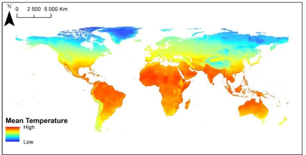
Figure 1. Worldwide mean annual temperature (from WorldClim; www.worldclim.org)...13
Figure 2: Latitudinal shifts in major habitats during climatic oscillations occurred in Africa since the Last Glacial Maximum until present. Adapted from Adams and Faure 2004………17
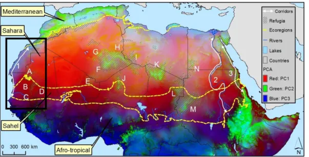
Figure 3: Environmental variability in North Africa derived by Spatial Principal Component Analysis (SPCA). The West Sahara region comprised within the black rectangle corresponds to the proposed corridor. Adapted from Brito et al., 2014……….20
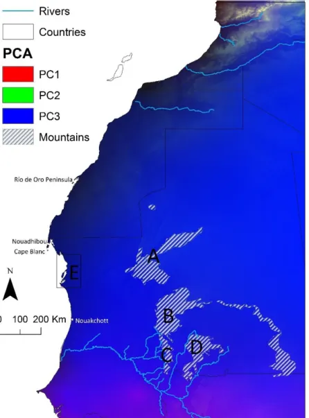
Figure 4: Environmental variability in West Sahara derived by Spatial Component Analysis (SPCA). Main rivers and mountains are represented………..…21
Figure 5: Variation of maximum temperature (Max Temp) and annual precipitation (Ann Prec) in the West Sahara through time...22
Figure 6: Known distributional ranges of the study species in North Africa, with photography of a representative individual: A) T. annularis, B) T. hoggarensis, C) T. parvicarinata and D) T. chazaliae. Adapted from Bons & Geniez, 1996 and Trape et al., 2012………..26
Figure 7: Spatial distribution of the distributional records and samples used in this thesis. ……….………...35
Figure 8: Bayesian phylogenetic tree of the Tarentola species based on 388 bp of the 12S gene. ………..43
Figure 9: Individual analyses for Tarentola annularis……….………46
Figure 10: Individual analyses for Tarentola chazaliae…….………..…47
Figure 11: Individual analyses for Tarentola hoggarensis……….………48
Figure 12: Individual analyses for Tarentola parvicarinata…...………..49
Figure 13: Response curves for the bioclimatic variables most related to the distribution of Tarentola. ………..50
Figure 14: Sum of stable areas for all species. ………60
Table Index
Table 1: Sample sizes for building ENMs for each species. Total: total number of observations;
Training: number of observations used to construct the model; Validation: number of observations used to test the models……….34
Table 2: Climatic variables used for building the Ecological Niche-based Models of Tarentola,
with units and range of variation for current conditions. Table 2: Climatic variables used for building the Ecological Niche-based Models of Tarentola, with units and range of variation for current conditions……….36
Table 3: Number of observations to train and test models for each species, average and standard
deviation (SD) of training and test AUC derived from the 20 replicates, minimum training presence logistic threshold (MTP), and average percent contribution (with standard deviation) of each variable in the models. Most important variables are marked (*)………..45
Table 4: Genetic distances (diagonal left) between the lineages of each study species with
standard deviation (diagonal right). Numbers in red represent the genetic distances between the lineages of each species. TA stands for T. annularis, TCA, TCB and TCC for lineages A. B and C of T. chazaliae, THA, THB, THC and THD for lineages A, B C and D of T. hoggarensis, and TPS, TPC and TPN for lineages S, C and N of T. parvicarinata……….54
1. Introduction
1.1. Climate
Climate comprises all the aspects of the hydrosphere-atmosphere-land system, with all their complex interactions and feedbacks, in a limited time scale (Quante, 2010). Since the origin of life about 3.5 billion years ago, Earth’s climate has oscillated due to both external (changes in solar radiation) and internal factors (changes in orbit, tectonic plates and volcanoes) as well as life itself (e.g. through photosynthesis, organisms altered the composition of the atmosphere). As life continually evolved, it became more involved in climatic cycles, such as water and carbon, changing the energy budget of the Earth, and ultimately impacting life itself (Quante, 2010). These climatic changes over time led to diversification processes, while spatial variability, in conjunction with landscape features, shaped species distributions (Slatkin, 1987; Brown and Lomolino, 1996).
1.1.1. Climate variation in space and time
Climatic conditions greatly vary all over the world (e.g. temperature; Figure 1) and this is primarily the result of the interaction between solar radiation (which is higher between the tropics), atmospheric circulation and oceanic currents (Rickelfs, 2008).
Topographic and geographic features can also affect climate at a local or regional scale. For instance, mountains usually present higher variation in temperature and more precipitation levels than surrounding lowlands, while coastal areas tend to have less variation in temperature than the interior, as well as more precipitation (Rickelfs, 2008). Through time, climate has also changed considerably. For instance, during the Cretaceous, Earth’s temperature was higher than at the present (Quante, 2010). At the end of this epoch, however, a decline in the concentration of CO2 in the atmosphere led
to a cooling of the planet (Quante, 2010). The Arctic ice cap started to grow, marking the beginning of the Pleistocene ca. 2.4 Mya (Damuth, 1975; Hewitt, 2000). The Pleistocene period is characterized by strong oscillations in climate, alternating between glacial periods, where the ice sheets spread through most of northern landmasses (i.e. North America, North of Europe and Siberia), and warmer interglacial periods, where the ice cap was restricted to northernmost latitudes (i.e. Antarctica and sometimes Greenland) (Quante, 2010). Tropical and temperate regions were compressed towards the equator during glacial periods and an increased aridity lead to a reduction of tropical forests and expansion of deserts (Hewitt, 2000, 2004). The oceans, covering about two-thirds of the planet’s surface, had a strong influence on these oscillations (Quante, 2010) and were also affected by them, as with the spread of the glaciers, sea level was considerably reduced (Hewitt, 2000). These oscillations have been shown to have occurred in cycles of 100, 41 and 21 thousand years that result from the complex interaction of changes in the Earth’s orbit, tilt and axial wobble, and affected the amount of energy received from the sun. In turn, a big part of the energy received is transported by the oceanic currents, allowing for fast and global climate changes (Zagwijn, 1992; Hewitt, 2000).The transition between the Last Glacial Maximum and the Holocene period about 11,700 years ago (Walker et al., 2009) was dramatic. Ice caps started to retreat rapidly, and a large volume of water flooded the land and formed many lakes, as well as created continental islands and reshaped the coastal line (Quante, 2010). Around the Middle Holocene (about 6,000 years ago), solar radiation was 8% higher and lower than today in the peak of summer and winter respectively in the northern hemisphere. This caused and increased ocean evaporation, resulting in higher continental precipitation (Quante, 2010).
Information on past climate comes from many sources. Ice cores can give detailed climatic information over the last 400.000 years, though most are only informative for the last 125.000 years. Through these ice cores, annual analyses of gases, isotopes and acidity can be performed (Seierstad et al., 2014). Sediment analyses can also give information on distant climate, though in a more indirect way and
with less resolution. It is also more restricted to humid habitats, as sedimentation is less likely to occur in dry habitats (Kröpellin et al., 2008). Pollen records also provide invaluable indirect evidence, as most can be identified at the species level, and thus, detailed habitat reconstructions of past times can be performed (Whitmore et al., 2005; e.g. Russia, Tarasov et al., 2005; Central Africa, Jolly et al., 1998; South Africa, Palazzesi and Barreda 2012). Fossils can also be informative, but their scarcity and difficulty of identification of some fragments can limit their usefulness (Williams et al., 1998; Hewitt, 2000).
1.1.2. Current patterns of biodiversity
Biodiversity is not homogeneously distributed across the Earth (Brown and Lomolino, 1996). Tropical regions harbor the highest levels of biodiversity in most of the taxa, while Polar Regions the lowest (Gaston, 2000). Such latitudinal gradient occurs both at a regional and continental scales (Hillebrand, 2004). Topographical gradients are also frequent and usually mountain ranges harbor higher diversity than flat areas (Simpson, 1964). Islands are also regions of great scientific interest, as due to their isolation they usually present a unique species assemble (MacArthur and Wilson, 2015).
Current distributional patterns of biodiversity can be mostly attributed to climatic oscillations that occurred in the Late Pleistocene (Carnaval et al., 2009). In general, during the unfavorable periods of these climatic oscillations, most species went extinct or their ranges became reduced in large parts of their distributional area. But some were able to survive in specific climatic suitable areas (i.e. refugia), subsequently expanding during favorable conditions, while others were able to disperse to new locations (Hewitt, 2000). Additionally, some species were able to persist in their previous range by adapting to the new climatic conditions through niche shifts (Hoffmann and Sgrò, 2011). However, landscape features, ocean currents and latitude regionally modulated the global patterns of climate. Futhermore, each species reacted differently to climate changes owing to their own ecological requirements and life-history traits (Hewitt, 2000).Species with different affinities responded differently to the same climate changes (Hewitt, 1999), although some were able to adapt to the new conditions (Hoffmann and Sgrò, 2011). In temperate regions, warm adapted species experienced range contraction during cold periods, expanding again during warmer periods (e.g. species with Mediterranean affinity; Hewitt, 2004), while cold or mountain adapted species expanded their ranges
during cold periods and contracted in warm ones (e.g. species with Euro-Siberian affinity; Hewitt, 2004). A similar process likely happened with tropical species, albeit these expansions and contractions occurred in a lesser geographic extent (Hewitt, 2004). During humid periods, usually associated with cooler climate, xeric species likely became isolated and diversified, expanding during dry periods (e.g. Chalcides, Carranza et al., 2008; Brito et al., 2014). Contrarily, mesic species expanded during humid periods, contracting and becoming isolated when climate became dryer (e.g. Taterillus, Dobigny et al., 2005; Hewitt, 2000, 2001). The effects of climatic oscillations on biodiversity patterns have been extensively addressed in many regions of the world (e.g. in Europe and North America; see Murphy and Weiss, 1992; Taberlet et al., 1998; Hewitt, 2000, 2001; Weiss and Ferrand, 2007; Sommer and Zachos, 2009), but research is lacking for remote regions (Brito et al., 2014).
1.2. The Sahara-Sahel
North Africa is a region of great biogeographic interest. The great diversity of habitats, heterogeneous landscapes and complex geologic and climatic histories all contribute to the biodiversity uniqueness of this region (Le Houérou, 1997; Comes 2004; Sayre et al., 2013).
The Sahara desert and the adjacent arid region Sahel cover most of North Africa and correspond to two of the biggest ecoregions of the continent (about 11,230,000 km2;
Olson et al., 2001). These areas present a high diversity of topographic features, as well as a heterogeneous climate resulting from spatial variability in both temperature and precipitation. The transition between the Paleartic and Afrotropical biogeographic realms correspond to the limit between the Sahara and the Sahel (Olson et al., 2001). This leads to great latitudinal variation in species distributions and high local biodiversity (Dumont et al., 1982; Le Houérou, 1992; Brito et al., 2016).
Species inhabiting these regions present unique adaptive features to cope with the severe environmental conditions, such as scarce and unpredictable food and water, and extreme temperatures and solar radiation (see Brito et al., 2014). Species ranges are usually under strong climatic control, and many species have patchy distributions. The evolutionary processes that led to the adaptation of organisms to such extreme environments also led to high rates of endemism (Ward, 2009).
The Sahara was not always a desert. Desertification is estimated to have begun about 7 million years ago in Chad (Schuster et al., 2006; Zhang et al., 2014), or between 6 and 2.5 million years ago in western areas (Swezey, 2009). Since its formation, this region has experienced, and is still experiencing, strong climatic fluctuations resulting from feedbacks between precipitation and vegetation cover (Wang et al., 2008; Clausen, 2009). Since the Pliocene (5.3 Mya), the Sahara-Sahel went through several dry-wet cycles, at least eight to ten in the past 125,000 years (Le Houérou, 1997). These shifts greatly modified geomorphic processes, which was subsequently accompanied by changes in fauna and flora. During the humid periods, afro-tropical habitats expanded northwards (Figure 2), probably followed by an expansion of afro-tropical species such as fishes (e.g. Barbus macrops, Clarias anguillaris Trape, 2009), amphibians (e.g. Hoplobatrachus occipitalis; Amietophrynus xeros Tellería, 2009) and reptiles (e.g. Echis leucogaster; Crocodylus suchus Trape and Mane, 2006; Brito et al., 2011a). The Sahara-Sahel was covered by a dense river network with multiple basins and large lakes (Drake et al., 2011). These wetlands were covered by extensive vegetation (Gasse, 2000; Kröpelin et al., 2008). The last wet period occurred between the Late Pleistocene (14,500 ya) and the Middle Holocene, ending between 6,000-5,000 years ago, when aridity began to increase significantly, with mesic communities disappearing and lake levels
Figure 2: Latitudinal shifts in major habitats during climatic oscillations occurred in Africa since the Last Glacial Maximum until present. Adapted from Adams and Faure 2004.
decreasing (Foley et al., 2003; Holmes, 2008). Current patterns of biodiversity in the Sahara-Sahel resulted from these climatic and land-cover oscillations (see Brito et al., 2014).
1.2.1. Evolution in Sahara-Sahel
Despite recent studies in the region, evolutionary processes in the Sahara-Sahel remain largely unknown. Phylogeographic studies are revealing that diversification and speciation in the Sahara-Sahel are most likely related to spatial and temporal variation of the desert extent (Brito et al., 2014). While the southern limit of the Sahara moved significantly during the Quaternary (1-6Mya), the northern limit appears to have retained approximately the same position (Le Houérou, 1997). The onset of the Sahara itself is likely to have created vicariance in a North-South axis, affecting diversification processes in many species. For example, the separation of two Macroscelidae mammals has been linked to the formation of the Sahara, with no apparent secondary contact ever since (Douady et al., 2003). Carranza et al., 2008 have also linked the origin and divergence of skinks and the age of the Sahara.
The occurrence of several cycles of wet-dry periods also had a profound impact on diversification processes of biota in the Sahara-Sahel region. These oscillations are estimated to have occurred in cycles of 100,000-20,000 years (Le Houérou, 1997), greatly shifting the range of savannah and desert environments and constrained the distribution and genetic structure of many species (Brito et al., 2014). The many cycles of expansions and contractions resulted in contrasting patterns. Unsuitable climatic periods would have led to divergence due to absence of gene flow between refugia (e.g. Guillaumet et al., 2008) while dispersal and gene flow would occur along geographical corridors during suitable climatic periods (e.g. Gaubert et al., 2012). For instance, Dobigny et al., 2005 showed that during the last million years, the West African Taterillus gerbils were likely restricted to refugia during dry periods and expanded in wet periods while being constrained by rivers, which probably led to parapatric species distribution and genetic evidence of bottlenecks. Similarly, the arid-adapted Stenodactylus geckos, which are present throughout Arabia and North Africa, exhibit high genetic diversity, with geological events and climatic instability as the main probable drivers of their divergence (Metallinou et al., 2012). Nonetheless, despite these strong variations, mountains likely acted as refugia for many species since allowed vertical shifts of environmental
conditions and thus, population persistence through time (Messerli and Winiger, 1992; Gonçalves et al., 2012, Velo-Antón et al., 2014).
The Sahara-Sahel is an excellent model for studying the effects of extreme climate oscillations on biodiversity dynamics. However, such studies are still scarce, especially for species truly adapted to its arid conditions. Studies on patterns and processes in the region have largely been neglected and the role of landscape and climate remains poorly understood (Brito et al., 2014).
1.2.2. Trans-Saharan biodiversity corridors
One pattern that emerges is that the Sahara desert effectively acts as a barrier to many species that are not fully adapted to arid conditions. However, there is plenty of evidence that many non-Saharan species persist in refugia throughout the desert (see Brito et al., 2014). This suggests the existence of biodiversity corridors (narrow strips of habitat that connects two or more suitable patches; Rickelfs, 2008) across the Sahara (Figure 3), at least during wet periods. Brito et al., 2014 reported that many of these isolated populations exist in restricted habitats within oases and mountains that are currently surrounded by sandy and rocky areas. But in the past, these areas were probably connected by savannah-like habitats during humid periods (Gasse, 2000; Kröpelin et al., 2008), therefore forming a network of biodiversity corridors in a North-South axis (Dumont, 1982; Drake et al., 2011). Most of these corridors disappeared during dry periods, as they did during the present, but others may have persisted even during dry periods. The Atlantic and Red Sea coasts, as well as the Nile River (see Figure 3) stand out as the most probable ones (Brito et al., 2014). The Nile River has been regarded as a long and narrow oasis that prevailed at least since the last glaciation (Krings et al., 1999). The Atlantic and Red Sea coasts are influenced by the sea proximity, and thus have a milder climate (Brito et al., 2009; Brito et al., 2011b). There have been some studies addressing the Nile River and the Red Sea coast as biogeographic corridors, mainly for the dispersal of hominins (e.g. Drake et al., 2011). However, no study addressed the climatic stability of the Atlantic Sahara as a corridor over time, linking such stability to the genetic structure of species.
1.2.3. The West Sahara region
The West Sahara is a variable region in terms of climatic and habitat factors. At this respect, three units can be currently identified (Figure 4):
1. The Atlantic Coastal Desert, consisting of a narrow strip of land along the Mauritanian and Western Saharan coast, extending just 40 km inland, which has being previously identified as a WWF ecoregion (Olson et al., 2001). It comprises the westernmost part of the Sahara and is characterized by low altitude (maximum of 200 m) and sandy or gravy substrate (Olson et al., 2001). The climate is hot and dry, with low and sporadic rainfall, but mists from the Atlantic are common, bringing humidity when condensing (Olson et al., 2001). Desertification in this region is thought to have begun more recently than in other areas (Swezey, 2009). Nevertheless, it was also subject to several dry-wet cycles, albeit less intense than in more inland areas due to the influence of the sea. One important landscape feature, however, is that during the Last Glacial Maximum sea levels decreased, and thus terrestrial habitat increased.
2. Inland regions to the Atlantic Coastal Desert, suffer less influence from the sea, and are thus characterized by increasing warmer temperatures and low precipitation.
Figure 3: Environmental variability in North Africa derived by Spatial Principal Component Analysis (SPCA). The West Sahara region comprised within the black rectangle corresponds to the proposed corridor. Adapted from Brito et al., 2014.
Annual rainfall is usually between 100 and 200 mm, increasing from north to south, but droughts lasting several years are not uncommon. It also has low altitude and the substrate is mostly composed of sand. Some more arid resistant plant species of Sahelian origin can be found in this region, such as Acacia trees (Olson et al., 2001).
3. Inland rocky areas, such as the mountains of Gueltat Zemour and Adrar Soutuf in Western Sahara, and the Mauritanian mountains of Adrar Atar, Tagant and Assaba. These mountains have moderate altitude, ranging from 300 to 900 meters, and the substrate is mostly rocky. They also present a unique climate, with an increase of humidity comparing to the surrounding areas, especially in the southern mountains. This
Figure 4: Environmental variability in West Sahara derived by Spatial Component Analysis (SPCA). Main rivers and mountains are represented; A: Adrar-Atar; B: Tagant; C: Assaba; D; Affolé; E: Parc National Banc du d’Arguin.
allows the persistence of relict populations of both Mediterranean and Sahelian taxa in the middle of the desert (Olson et al., 2001).
In the West Sahara, climate has importantly varied through the Late Pleistocene (Figure 5). Generally, in the Last Inter Glacial (LIG, 120 kya), maximum temperature and annual precipitation were higher than in the present, especially in more inland regions. During the Last Glacial Maximum (LGM, 21 kya), maximum temperature and annual precipitation decreased. In the Middle Holocene (MidHol, 6 kya), climate became slightly warmer and wetter. Maximum temperature in the Atlantic Coastal Desert remained reasonably constant, being slightly lower during the LGM. However, annual precipitation varied greatly, being moderately high during the LIG and decreasing towards the present. More inland areas suffered greater oscillations, especially in precipitation. Maximum temperature was higher during the LIG, decreasing towards the LGM and remaining approximately constant until the present. Annual precipitation was significantly higher during the LIG, greatly decreasing towards the LGM. In the Middle Holocene, annual precipitation increased, but then decreased again towards the present. In mountainous areas, similarly to coastal regions, climate was more constant, and generally maintaining a cooler and wetter climate than the surrounding areas. During the LIG climate was warmer, with temperature decreasing towards the Middle Holocene, slightly increasing in the present. Annual precipitation remained more or less constant, only being slightly higher in the Middle Holocene.
Figure 5: Variation of maximum temperature (Max Temp) and annual precipitation (Ann Prec) in the West Sahara through time. For the LGM only one GLM is represented, corresponding to CCSM (Community Climate System Model) scenario. Climatic variables were retrieved from WorldClim (www.worldclim.org).
The effect of climatic variability in the West Sahara biodiversity remains poorly understood. Many species with continuous distribution in either north or south of the West Sahara desert present isolated populations on the other side and some even have relict populations in suitable patches in the mountains thus, suggesting this region as a corridor (Brito et al., 2014). When distributional patterns of taxa inhabiting the West Sahara are analysed, four main patterns of species distributions can be differentiated:
1) Species showing a disjoint distribution
Some species can be found both north and south of the West Sahara, with no connection in between. This is the case of some Afrotropical species such as the puff adder Bitis arietans, which inhabits a range of semi-arid open habitats extending throughout sub-Saharan Africa, and north of the Sahara in isolated populations in southwest Morocco. This species presents a distinct West African clade, with indivisuals from both north and south of the Sahara grouped together (Trape and Mane, 2006; Barlow et al., 2013).
2) Species endemic to the coastal region
Some species are endemic to the Atlantic coastal desert, having a restricted distribution near the Atlantic coast and only expanding a few kilometers inland. For instance, the small lizard Acanthodactylus aureus exists only along the Atlantic Sahara (Crochet et al., 2003; Trape et al., 2012), but recent inferences on its genetic variability indicated high levels of structuration along it (Lopes, 2014).
3) Species with almost continuous distributions from one realm to another
Some species are typically Mediterranean and expand to the Sahara and sometimes Sahel, while others are major sub-Saharan but can be found in Saharan mountains. The Mediterranean snake Psammophis schokari exemplifies the first case as it is distributed across the Mediterranean in North Africa and penetrates along the western Sahara coast, reaching Mauritania (Trape and Mane, 2006; Rato et al., 2007). Exemplifying the second case, the North African Agama boulengeri lizard which is Sahelian, but colonized the Sahara, presumably during wet periods, diversifying during dry ones; currently, presenting north-south genetic sub-structure (Trape et al., 2012; Gonçalves et al., 2012). Crocodylus suchus is also another example (see Trape et al., 2012), thought to have colonized the Mauritanian mountains from southern ranges during
wet periods, with subsequent isolation when climate became drier (Velo-Antón et al., 2014).
4) Species with widespread distributions in arid conditions
Species adapted to arid conditions typically have a widespread distribution throughout the Sahara (Brito et al., 2014). These species present adaptations to cope with extreme climate, and thus are expected to have reacted in an opposite manner than non-Saharan species. For instance, the arid adapted Cerastes vipers are widespread throughout the Sahara (Trape and Mane, 2006), including one species adapted to rocky and another to sandy areas (Brito et al., 2011b). Similarly, Acanthodactylus dumerili (including the synonymous A. senegalensis; Lopes, 2014) is also widespread, though it avoids the central areas of the Sahara (Trape et al., 2012). While no genetic studies exist for the viper species, A. dumerili was found to have two lineages, with one distributed throughout all the southern range and another apparently restricted to Morocco (Lopes, 2014).
These four patterns of species distribution described here are apparently related to the distribution of climatic variability. For instance, the coastal desert corresponds to an area of milder temperatures than the interior regions (Olson et al., 2001). This particular climate, derived from the proximity of the sea, likely restricted endemic species to the coastal desert. When comparing current climatic patterns in the region with predictions of past climate, both temperature and precipitation are more variable in inland areas, while remaining more constant near the coast (Fig. 4). Similarly to other African mountains (Messerli and Winiger, 1992), Saharan mountains also present lower temperatures than the surrounding low altitude areas, as well as higher precipitation (Olson et al., 2001). Mountains likely acted as climatic refugia favoring the persistence of species not adapted to arid conditions during dry periods as the current. For example, Vale et al., 2015 showed that Mauritanian gueltas, despite their small size, are important micro-hotspots of biodiversity. All of these inferences raise the question of whether climatic stability in the different regions of the West Sahara resulted in the persistence of ecological corridors through which species could cross the Sahara even during unfavorable periods.
1.3. Species model: Tarentola
Reptiles constitute good models to infer the role of climatic variability on biogeographical patterns. Being ectothermic, reptiles are dependent on environmental temperature, presenting several behavioral, physiological and anatomical traits that allow them to regulate their internal temperature with low energy costs (Shine, 2005). As a result, reptiles were highly susceptible to the climatic oscillations of the Pleistocene, and their low dispersal capacity hindered their ability to track suitable habitat (Araújo and Pearson, 2005).
In this thesis, I used geckos of the genus Tarentola to infer the role of climatic oscillations as drivers of their genetic structure. The genus Tarentola (Fam. Phyllodactylidae) comprises 21 species, distributed across North Africa, coastal regions of the Mediterranean Sea, Macaronesia and the West Indies (Cuba and Bahamas; Rato et al., 2012; TRD, 2016). All species present low inland dispersal capacity and are morphologically similar, with a large head, short plump body, slender limbs and short tail. They form a monophyletic clade, being phylogenetically close to Pachydactylus and Hemidactylus (Carranza et al., 2002). The genus is formed by two main clades, one containing species as Tarentola annularis, T. chazaliae and T. ephippiata, and the other the likes of T. mauritanica and T. deserti, T. boehemei and T. fascicularis (Rato et al., 2012). The origin of the genus goes back to the Miocene with the split between the two main clades occurring in this period (Rato et al., 2012). Furthermore, high genetic divergence has been found within T. mauritanica, suggesting several cryptic species (Rato et al., 2015). However, no study addressed in detail the genetic structure within the other Tarentola species.
Four Tarentola species inhabit the West Sahara (Schleich et al., 1996, Trape et al., 2012):
1) Tarentola annularis (Geofrey-St-Hilaire, 1827) is a relatively large species, with a maximum snout-vent length (SVL) of 14 cm, and can be identified by the presence of four white spots in the shoulder region arranged in a square (Figure 6A). This species has a widespread distribution from the Western coast to Somalia and Egypt, and can be found in rocky desert plains along the Sahel and some parts of the Sahara (Figure 6A; Trape et al., 2012).
Figure 6: Known distributional ranges of the study species in North Africa, with photography of a representative individual: A) T. annularis, B) T. hoggarensis, C) T. parvicarinata and D)
2) Tarentola hoggarensis (Werner, 1937) is relatively small, with a maximum SVL of 8.2 cm and characterized by four transversal dark bands in the dorsum (Figure 6B). It inhabits arid areas of Western Sahel and part of the West Sahara (Figure 6B), where Acacia trees are more or less abundant. It was previously considered as a subspecies of T. ephippiata, but it was more recently elevated to species level (Trape et al., 2012). Another former subspecies of T. ephippiata recently elevated to species level is T. senegambiae. This species is larger, with a maximum SVL of 13 cm, and is restricted to Senegal, Gambia and Guinea-Bissau. It is typically arboreal, though it can be found in buildings and walls (Trape et al., 2012). However, molecular studies are lacking to confirm the validity of these species and to determine their relation with T. ephippiata and T. hoggarensis.
3) Tarentola parvicarinata (Joger, 1980) has a maximum SVL of 9.7 cm, a lighter coloration and large tubercles in the tail (Figure 6C; Trape et al., 2012). No molecular study has included this species, and thus its phylogenetic relationship with the remaining Tarentola species remains unknown. This species is found almost excusively in mountain regions with rocky substrate, namely in Mauritania and Mali (Figure 6C; Trape et al., 2012).
4) Tarentola chazaliae (Mocquard, 1895) is smaller, with a maximum SVL of 7.4 cm, and a disproportionately large head (Figure 6D). It is sometimes called helmeted gecko because it presents a row of conical occipital tubercles that resemble a helmet. Previously considered to be part of the genus Geckonia, but an integrative study with morphological and molecular markers revealed that it is in fact a Tarentola (Carranza et al., 2002). This species is endemic to the Atlantic Sahara, inhabiting cooler and more humid habitats than the other species, and extending their distribution just a few kilometers inland (Figure 6D). It prefers sandy and rocky soils with large deposits of vegetation (Trape et al., 2012).
By apparently displaying distinct ecological/habitat requirements, these four Tarentola species offer an interesting biological system to investigate the effect of Pleistocene climatic oscillations on their genetic structure across the West Sahara. The four species are expected to follow one of the continuous distributional patterns previously described: (i) T. annularis would follow the pattern of the widespread arid-adapted species like A. dumerilli and thus, genetic structuration should be low; (ii) T.
chazaliae is expected to follow the endemic distribution pattern, similar to A. aureus and thus, genetic structure should be high; and (iii) T. hoggarensis and (iv) T. parvicarinata would display an almost continuous distribution pattern, being both Sahelian species penetrating northwards but adapted to different habitats (i.e. Acacia trees the former, mountainous areas the latter). These species should exhibit similarities with A. boulengeri or C. suchus, for instance, and thus genetic structuration would be dependent on specific habitat characteristics.
1.4. Genetic and ecological approaches
Combining phylogeographic and Ecological Niche-based Modelling to study patterns of biodiversity has seen recent attention, as both approaches complement each other well (Kozak et al., 2008; Alvarado-Serrano and Knowles, 2014).
Phylogeography is the integration of several genetic data sources in a geographic context in order to understand the relationship between geographic features and species distributions (Hickerson et al., 2010). The choice of molecular marker is central to phylogeography, and different markers are used to help answering different questions. Each molecular marker has different rates of evolution and can be subjected to different selective pressures. Thus, working with mitochondrial (mt) or nuclear DNA (nDNA) might yield different results (e.g. Wan et al., 2004). The choice of marker will depend on the question being addressed. For example, microsatellites are suitable for studying recent dynamics such as at a population level due to their fast evolutionary rate (Goldstein and Schlotterer, 1999), while coding nDNA is more conservative, being more indicated to infer relations among distant taxa, as genera or families (Zhang and Hewit, 2003). MtDNA is less conservative, thus being better suited to infer both interspecific and intraspecific relationships (Wan et al., 2004). However, mtDNA is maternally inherited, reflecting only the matrilineal evolutionary history. The effective population size of mtDNA is also only a fourth of nuclear markers, resulting in a faster lineage sorting and allele extinction rates, leading to a potential oversimplification of phylogenetic relations and underestimation of genetic diversity (Zhang and Hewitt, 2003). Within the same class of markers (e.g. mtDNA), some variation exists as far as mutation rate is concerned, with different markers being suitable to address different time scales (Wan et al., 2004). MtDNA is the most commonly used tool for phylogeographic analyses.
Genetic data has some shortcomings when trying to build phylogegraphic hypothesis. For example, phylogeographic approaches are limited when addressing “where” biogeographic events occurred. Genetic data can indicate population expansion or contraction, but provides limited information on where those populations occurred when they were large or small (Peterson, 2009). This question, however, can be independently inferred with Ecological Niche-based Models (ENMs). ENMs correspond to a series of methods that aim to determine the ecological niche of a species (fundamental vs. realized; see Sillero, 2011) and its potential distribution (Peterson, 2011). Although hybrid approaches exists, ENMs can be divided into correlative and mechanistic approaches. Correlative approaches aim to determine the realized ecological niche of a species (i.e. the Grinnellian niche, sensu Soberón, 2007) by associating its distribution with the environmental conditions of where the species occurs. On the other hand, mechanistic approaches try to spatially map different aspects of the fundamental ecological niche of species, linking functional traits with the environmental conditions that species experiment along their ranges (Wiens et al., 2009; Alvarado-Serrano and Knowles, 2014). Mechanistic approaches, however, require detailed information on the physiological tolerances of the organisms, for instance, which remain unknown for most species. Thus, most studies use correlative approaches as data on species presence (or absence to a lesser extent) is widely available (Elith et al., 2010; Alvarado-Serrano and Knowles, 2014).
ENMs are not exempt from assumptions and uncertainties either. For instance, when building the models, it is impossible to measure all the variables that potentially influence the niche of a species (i.e. the Fundamental niche) and thus there is always the risk of a species niche being determined by unmeasured variables (Wiens et al., 2009). Another assumption is that species are in equilibrium with the environment, that is, the suitable habitat is fully occupied (Soberón and Peterson, 2005). However, a species may not be present in a suitable patch of habitat if a recent disturbance eradicated it from that area or if a patch only became available recently and the species was not yet able to colonize it (Wiens et al., 2009). On the other hand, some individuals might be found in a patch no longer suitable for the species due to having high longevity (such as with some plant species; Foden et al., 2007). To assume equilibrium with the environment, it is also necessary to assume that individuals are capable of dispersing to suitable locations (Pearson and Dawson, 2003). However, species with low dispersal rates may not be able to track the shifting suitable habitat and must either adapt to the new conditions, or survive in refugia (e.g. Velo-Antón et al., 2015). ENMs also assume
that each species react to the environment independently, with their niches not being influenced by biotic interactions (Wiens et al., 2009). This has been shown not to be true (Araújo and Luoto, 2007), as by definition, a species realized niche is restricted by the interactions with other species (Soberón, 2007) but remains an overwhelming challenge for most studies (Wiens et al., 2009; Kissling et al., 2012). ENMs also assume that the niche of a species is conserved, that is, it is an immutable characteristic of a species, thus remaining constant through space and time. This assumption justifies the possibility of extrapolating models to different time periods (Wiens and Graham, 2005). Finally, sampling the complete climatic niche where a species is able to thrive is considered one of the main factors affecting the reliability of SDM predictions. To measure the true adaptive potential of a species, it is necessary to sample the entire climatic niche of said, minimizing the uncertainties associated when projecting to a different time period (Thuiller, 2004; Wisz et al., 2008; Nogués-Bravo, 2009; Barbet-Massin et al., 2010; Martínez-Freiría et al., 2016).
Some uncertainties must also be taken into consideration. Some violate the assumptions, but others have different sources. For instance, climatic conditions for the past cannot be directly measured, and must be derived. Different methods take into consideration different parameters, and predict different conditions. Furthermore, there are several algorithms used to construct ENMs, which deal with the assumptions differently, and can lead to different predictions. The quality of the data used can also have and important impact on the ENMs. The records of species occurrence need to be reliable, as well as the data on the environmental conditions. Finally, the scale at which the ENMs are constructed, need to be concordant with the scale at which the environmental variables affect the niche of the species. For example, climatic variables can define the niche of a species at a coarse scale, but at a finer scale, other factors, such as species interaction or land cover can have a bigger impact. Acknowledging the assumptions and uncertainties of ENMs is essential to correctly interpret ENMs (Wiens et al., 2009; Alvarado-Serrano and Knowles, 2014; Martínez-Freiría et al., 2016).
Phylogeographic and ENM tools complement each other well. ENMs can be used to interpret the patterns of genetic variations by visually comparing the geographic distribution of the genetic patterns with the projected distribution of a species (Alvarado-Serrano and Knowles, 2014). For example, Martínez-Freiría et al., 2015 identified northwest Iberia as climatic refugia for Vipera seoanei based on mtDNA genetic pattern, which was corroborated by an ENM approach that identified the same area as suitable, both in the present and in the past. Habitat suitability can also be converted into probable
migration routes that can be compared to genetic distances (McRae, 2006). On the contrary, habitat suitability can be used to identify environmental barriers and compare with genetic breaks (e.g. Velo-Antón et al., 2015). When predicting species distributions for several time periods, it is possible to identify regions of environmental stability where species could have persisted over time. Carnaval et al., 2009 identified stable areas of tropical forests along the Brazilian coast for the past 21,000 years and compared them with genetic data for three frog species. As predicted, the populations from the stable areas presented a genetic signature that was different from the populations of unstable areas.
In this thesis I will take advantage of the combination of phylogeographic and ENM approaches to address evolutionary scenarios in West Sahara to try to understand whether this region served as a stable ecological corridor through time.
1.5. Objectives
This study aims to test the effect of climatic oscillations in the West Sahara by addressing the genetic structure of four species of the genus Tarentola with different ecological affinites. In order to fulfil this objective, two approaches will be used:
1 – Ecological Niche-based Modelling in order to understand how the study species respond to current and past climatic conditions in the Atlantic Sahara. This approach aims to answer the following questions: i) What are the climatic variables that most determine the distribution of the study species? ii) How suitable the West Sahara is for each species over time?
2 – Phylogeographic analysis to analyze the genetic structure of each study species. More specifically, this aims to answer two questions: i) Are the species genetically structured across the West Sahara? And if they are ii) how are the different lineages geographically distributed?
Overall, the genetic patterns and ENMs obtained for each species are compared within Tarentola and also with other reptile studies from the same geographic area in order to better understand the role of climate in shaping genetic structure in the West Sahara.
2. Methods
2.1. Study area
The study area covers the West Sahara region, spreading from Senegal to southern Morocco (13.5oN to 35.5oN) and thus including the Atlantic Sahara ecoregion,
and the adjacent inland region and mountain ranges of West Sahara and Mauritania until 6ºW (see Figures 4 and7).
The Fishnet tool from the Data Management Toolbox in ArcGIS (ESRI, 2006) was used to define the study area in a fashion that would include all the observations used and a 100 km buffer around them. A shapefile of the contour of the African countries was used to better visualize the spatial distribution of both the inputs (samples and climatic variables; see below) and the outputs.
2.2. Sampling
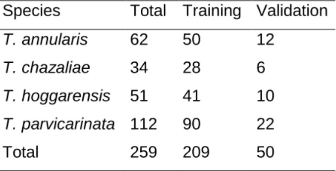
For Ecological Niche-based Models (ENM), 284 observations of T. annularis, 108 of T. chazaliae, 164 of T. hoggarensis and 339 of T. parvicarinata at 1 x 1 km resolution (WGS 1980 datum) were taken into account. Observations were gathered from fieldwork carried by BIODESERTS and collaborators (231 of T. annularis, 19 of T. chazaliae, 147 of T. hoggarensis and 339 of T. parvicarinata at at GPS precision), and from already published national atlases (e.g. Bons and Geniez, 1996; 53 of T. annularis, 89 of T. chazaliae and 16 of T. hoggarensis). In each species dataset, levels of spatial clustering were assessed with the Nearest Neighbor Index (NNI) from the Spatial Analyst extension in ArcGIS (ESRI, 2006), and a random removal of localities from clusters of each species occurrence was done to decrease it (e.g. Brito et al., 2011b; Martínez-Freiría et al., 2015). Finally, to perform ENMs, a low clustered distribution was obtained for each species (z-score=-1.642, NNI=0.894 for T. annularis with 62 presences; z-score=-1.627, NNI =0.854 for T. chazaliae with 34 presences; z-score=-1.646, NNI =0.883 for T. hoggarensis with 51 presences; z-score=-1.597, NNI =0.921 for T. parvicarinata with 112 presences; Table 1).
Table 1: Sample sizes for building ENMs for each species. Total: total number of observations; Training: number of observations used to construct the model; Validation: number of observations used to test the models.
Species Total Training Validation T. annularis 62 50 12 T. chazaliae 34 28 6 T. hoggarensis 51 41 10 T. parvicarinata 112 90 22
Total 259 209 50
For molecular analyses, tissue samples were available from South-Western Morocco, Western Sahara, Mauritania, Senegal and Mali (Figure 7). Samples were collected during fieldwork missions carried by the BIODESERTS group from 2004 to 2014. Each sample locality was recorded with a Global Positioning System (GPS) on WGS84 datum. From a total of 183 samples, 38 of T. annularis, 12 of T. chazaliae, 48 of T. hoggarensis and 72 of T. parvicarinata were selected to be sequenced in a way that would maximize the geographical coverage of the distribution of each species. The remaining 13 samples included other species, T. senegambiae (1 sample), T. boehmei (3 samples), T. deserti (2 samples), T. mauritanica (2 samples) and Tarentola sp (5 samples) were also sequenced and used as outgroups for genetic analyses (Figure 7).
2.3. Climatic variables
For current conditions, 19 bioclimatic variables were downloaded from WorldClim (http://www.worldclim.org/) at 30 arc seconds (~1 x 1 km) resolution (Hijmans et al., 2005). All variables were imported to ArcMap and cut to the study area using the Extract by Mask tool from the Spatial Analyst extension (ESRI, 2006). Spatial correlation among variables was assessed with the Band Collection Statistics tool from the Spatial Analyst extension and variables with high correlation (R > 0.70) were discarded. Three sets of variables were defined, all with low correlation. The variables in each set were visualized in ArcMap to check for spatial artifacts and inconsistencies (e.g. Kidd and Ritchie, 2000). The set chosen included six variables, three related to temperature and three to precipitation (Table 2), and thought to be biologically important for the study species (Rato et al., 2014).
Figure 7: Spatial distribution of the distributional records and samples used in this thesis. A) Total number of samples and records used for both the ecological and molecular approach. B) Distributional records per species used to build the ENMs. C) Tissue samples used for the molecular analyses, per species. Six samples of T. hoggarensis from Niger (see A) were also included in molecular analyses.
Table 2: Climatic variables used for building the Ecological Niche-based Models of Tarentola, with units and range of variation for current conditions.
Variable Units Range
Temperature Seasonality ºC 1092-8005
Min Temperature of Coldest Month ºC -14.4 - 18.9
Mean Temperature of Warmest Quarter ºC 11.0 - 36.9
Annual Precipitation mm 8 - 954
Precipitation of Driest Quarter mm 0 - 91
Precipitation of Coldest Quarter mm 0 - 662
For past climatic conditions, the same six variables were downloaded from WorldClim for three time periods: Last Interglacial (LIG; ~120,000–140,000 years BP; Otto-Bliesner et al., 2006), Last Glacial Maximum (LGM; ~21,000 years BP; Paleoclimate Modelling Intercomparison Project Phase II) and Middle Holocene (MidHol; ~6,000 years BP; Coupled Model Intercomparison Project #5. LIG variables were at 30 arc seconds resolution and accounted for one Global Circulation Model (GCM), NCAR-CCSM (Community Climate System Model; Otto-Bliesner et al., 2006). LGM variables were at 2.5 arc minutes (~5 x 5 km) resolution and corresponded to three GCMs: CCSM4 (Community Climate System Model, ver. 4, Collins et al., 2006), MIROC-ESM (Model for Interdisciplinary Research on Climate, ver. 3.2, Hasumi and Emori, 2004) and MPI-ESM-P (Max MPI-ESM-Planck Institute). These GCMs differ in temperature and precipitation, and in the West Sahara CCSM predicts the warmest climate, while MPI-ESM-P predicts the coolest, and MIROC predicts the wettest climate, while MPI-ESM-P predicts the driest. For the Middle Holocene, one GCM was retrieved: CCSM4 All variables were imported to ArcMap and cut to the study area using the Extract by Mask tool from the Spatial Analyst extension (ESRI, 2006). Finally, variables, both from present and for past conditions were exported from ArcMap to ASCII format in order to be used for the modelling analyses.
2.4. Lab Procedures
2.4.1. DNA Extraction
Samples consisted of tail tip tissue and were extracted with the EasySpin Genomic DNA Tissue kit (Citomed) following an adapted protocol (Annex A1). The quality and quantity of the DNA extracted was evaluated with an electrophoresis in a 0,8% Agarose gel stained with Gel Red in TBE 0,5x for 10-15 minutes at 300V. A Biorad Universal Hood II Quantity One 4.4.0 was used to visualize the gels exposed to UV radiation. According to this evaluation DNA extractions were proportionally diluted with ultrapure water to prevent possible inhibitions in the PCR reactions.
2.4.2. Marker selection
Several mtDNA markers were tested in order to obtain reliable information for phylogenetic/phylogeographic reconstructions. First, the cytochrome oxidase I (COI; Castaneda and de Queiroz, 2011) was initially chosen as it is a commonly used marker in phylogeographic studies due to its fast evolutionary rate (Knowlton and Weigt, 1998). However, after obtaining and aligning the first sequences, they presented a pattern typical of nuclear genes, with double peaks in many positions of the chromatogram. Thus, it was concluded that the selected primers were probably amplifying a nuclear pseudogene, and the marker was discarded. Another gene commonly used in phylogeographic studies was then selected: cytochrome-b (cyt-b; Kocher et al., 1989), and the same process of amplification and sequencing was performed. However, after aligning the first sequenced samples and building a preliminary Neighbour-Joining Tree, there were some inconsistencies between morphology and the tree obtained. The most glaring one is that T. chazaliae, which is morphologically quite distinct from the remaining species, did not form a unique clade, but was rather spread through the other clades, with one individual falling among T. annularis and the remaining within T. hoggarensis. This pattern could be due to a real evolutionary process, or could be as simple as a contamination. In order to distinguish between the two, another gene was necessary, and thus 12S (Kocher et al., 1989) was finally selected, which had already been successfully used in previous works with the genus Tarentola (e.g. Rato et al., 2012). As
this strange pattern was not found with 12S, contamination is unlikely, although more research will be needed to understand the unexpected pattern obtained in cyt-b.
2.4.3. Amplification and sequencing
Polymerase Chain Reactions (PCRs) were performed in a total volume of 10µl containing 5µl of MyTaq™ HS Mix (BioLine), 3µl of ddH2O, 0.5µl of each primer (forward
and reverse) and 1µl of template DNA. The PCR conditions are as follows: an initial denaturation at 95oC for 10 minutes, followed by 35 cycles of denaturation at 95oC for
30s, annealing at 52oC for 30s and extension at 72oC for 30s, and a final extension at
72oC for 10 minutes. Reamplification of samples that yielded too low amounts of product
was performed, using the same PCR conditions. A negative control was used in every reaction to check for contaminations. All PCRs were performed in a Biometra T100 thermocycler.
All PCR products were assessed by electrophoresis in 2% Agarose gels stained with Gel Red and with a mass DNA ladder (NZIDNA ladder V).
Part of the PCR products were purified and sequenced by a commercial company (Macrogen Inc, Netherlands). The remaining PCR products were purified using ExoSAP-IT® PCR clean-up Kit (GE Healthcare). The sequencing followed the BigDye® Terminator v1.1 Cycle Sequencing Kit (Applied Biosystems) protocol. The sequencing products were cleaned in sephadex and then rehydrated with ddH2O. Finally, the cleaned
sequencing products were read by capillary electrophoresis in a ABI3130xl Genetic Analyzer (AB Applied Biosystems).
2.5. Data analyses
2.5.1. Ecological Niche-based Models
A Maximum Entropy approach was used to build ENMs (Phillips et al., 2006). For this modeling technique, only presence data is required and has been shown that consistently performs well comparing with other methods (Elith et al., 2006), especially when the sample size is low (Hernandez et al., 2006; Wisz et al., 2008). Both the
presence records and the six climatic variables were imported to Maxent ver. 3.3.3 (Phillips et al., 2006). For each species, a total of 20 replicates were run with a random seed and 80-20% of the data was used for training-testing, respectively. In each replicate, the observations were chosen by bootstrapping, which allows sampling with replacement. These settings ensure that in each replicate a different and random subset of the data is used to train and test the models. Models were run with auto-features and the fit of each individual model was evaluated with the Area Under the Curve (AUC) of the receiver-operating characteristic (ROC) plot. Individual replicates were then projected to the different past climatic scenarios.
Individual models were averaged and standard deviation of presence probabilities used as a measure of prediction uncertainty (Buisson et al., 2010). Mean models reclassified in ArcGIS with the Reclassify tool of the Spatial Analyst extension into binomial suitable/unsuitable maps. The threshold used was the minimum training presence (MTP; Liu et al., 2013), which ensures that all presence records fall within the suitable area. All presence records were used to calculate this value on ArcGIS using the Extract Values to Table tool of the Geostatistical Analyst Toolbox. The reclassified models for each species were added with the Raster Calculator from the Spatial Analyst toolbox to build the stable suitable areas through time.
Variable importance for explaining the distribution of Tarentola geckos was determined by the average percent contribution to the models. This was done by both building models with only one of the variables, and models with all but that variable. Response curves of univariate models were visually examined to determine the preferred climatic conditions of each species (Phillips et al., 2006).
2.5.2. Phylogenetic analyses
Sequences were edited and aligned in Geneious Pro 4.8.5 (Drummond et al., 2009) using the Geneious alignment tool with default parameters. The alignment was then checked by eye to correct small misalignments and ambiguous positions. Every position that was not possible to determine the correct base, was considered as missing data (an N was edited into the alignment). The final alignment consisted of 388bp.
In order to estimate the root of the tree, two outgroups were used: one sequence of Hemidactylus turcicus and one of Pachydactylus turneri, both downloaded from GenBank. These two genera were chosen for being phylogenetically close to Tarentola
(Carranza et al., 2002). A total of 58 more samples were also downloaded from GenBank (see Annex A3 for accession numbers), comprising T. annularis (three sequences), T. chazaliae (four sequences), T. hoggarensis (four sequences), T. boehemei (15 sequences), T. desertii (22 sequences), T. fascicularis (two sequences), T. mauritanica (six sequences) and T. neglecta (two samples). All sequences of the four study species that were available were downloaded (no sequences were available for T. parvicarinata). For T. mauritanica, the six sequences represent all the African clades found by Rato et al., 2012. As the majority of the GenBank sequences were shorter than the ones obtained in the lab, the tips were filled with missing data in order to maintain the genetic information obtained for most of the sequences.
The 210 aligned sequences were collapsed into haplotypes with the online tool FABOX (Villesen, 2007) before further analyses, resulting in 94 unique haplotypes. In order to find the best-fitting model of nucleotide substitutions, JMODELTEST v.2.1.4 (Darriba et al., 2012) was used, and Bayesian Information Criterion (BIC) scores calculated to select the appropriate model (TrN + I + G).
Bayesian Analyses were performed in BEAST v.1.8.2 (Drummond et al., 2012). A lognormal relaxed clock was used, Yule process chosen as tree prior and ucld.mean Normal (initial value: 0.00827, mean: 0.00827, Stdev: 0.00162; according to Rato et al., 2012). Three independent Markov Chains of Monte Carlo (MCMC) runs of 80 million generations were performed, sampling at every 8,000 generations. The stationarity and convergence of the runs were evaluated in Tracer v.1.5 (Rambaut and Drummond, 2007), and values of Effective Sample Size (ESS) higher than 300 for all parameters were found. For building the final tree, the .log and .tree files of the three independent runs were combined with LogCombiner v.1.8.2 and summarized in TreeAnnotator v.1.8.2 (Drummond et al., 2012) with maximum clade credibility. FigTree v.1.3.1 (Rambaut, 2009) was used to visualize and edit the resulting tree.
2.5.3. Genetic structure
TCS v.1.21 was used to create haplotype networks with default parameters and a 95% threshold. To run this software, shorter sequences cannot be filled with missing data (Joly et al., 2007). As the sequences downloaded from GenBank were ~80bp shorter than the ones obtained in the lab, several mutating positions would be lost by cutting the sequences short. In order to evaluate the importance of this loss, two datasets