Large-scale parallelism for constraint-based local search:
the costas array case study
Yves Caniou, Philippe Codognet, Florian Richoux, Daniel Diaz, Salvador
Abreu
To cite this version:
Yves Caniou, Philippe Codognet, Florian Richoux, Daniel Diaz, Salvador Abreu. Large-scale
parallelism for constraint-based local search: the costas array case study. Constraints, Springer
Verlag, 2015, 20 (1), pp.30-56. <10.1007/s10601-014-9168-4>. <hal-01084270>
HAL Id: hal-01084270
https://hal.archives-ouvertes.fr/hal-01084270
Submitted on 18 Nov 2014
HAL is a multi-disciplinary open access
archive for the deposit and dissemination of
sci-entific research documents, whether they are
pub-lished or not.
The documents may come from
teaching and research institutions in France or
abroad, or from public or private research centers.
L’archive ouverte pluridisciplinaire HAL, est
destin´
ee au d´
epˆ
ot et `
a la diffusion de documents
scientifiques de niveau recherche, publi´
es ou non,
´
emanant des ´
etablissements d’enseignement et de
recherche fran¸
cais ou ´
etrangers, des laboratoires
(will be inserted by the editor)
Large-Scale Parallelism
for Constraint-Based Local Search:
The Costas Array Case Study
Yves Caniou · Philippe Codognet · Florian Richoux · Daniel Diaz · Salvador Abreu
Received: date / Accepted: date
Abstract We present the parallel implementation of a constraint-based Local Search algorithm and investigate its performance on several hardware plat-forms with several hundreds or thousands of cores. We chose as the basis for these experiments the Adaptive Search method, an efficient sequential Local Search method for Constraint Satisfaction Problems (CSP). After preliminary experiments on some CSPLib benchmarks, we detail the modeling and solving of a hard combinatorial problem related to radar and sonar applications: the Costas Array Problem. Performance evaluation on some classical CSP bench-marks shows that speedups are very good for a few tens of cores, and good up to a few hundreds of cores. However for a hard combinatorial search problem such as the Costas Array Problem, performance evaluation of the sequential version shows results outperforming previous Local Search implementations, while the parallel version shows nearly linear speedups up to 8,192 cores. The proposed parallel scheme is simple and based on independent multi-walks with no communication between processes during search. We also investigated a cooperative multi-walk scheme where processes share simple information, but this scheme does not seem to improve performance.
Keywords CSP · Local Search · metaheuristics · parallelism · implementation
Y. Caniou
JFLI & Universit´e Claude Bernard Lyon 1, France, E-mail: [email protected] Ph. Codognet
JFLI, CNRS / UPMC / University of Tokyo, Japan, E-mail: [email protected] F. Richoux
JFLI, CNRS / University of Tokyo, Japan & LINA, Universit´e de Nantes, France, E-mail: [email protected]
D. Diaz
Universit´e de Paris 1-Sorbonne, France, E-mail: [email protected] S. Abreu
1 Introduction
For a few decades the family of Local Search methods and Metaheuristics has been quite successful in solving large real-life problems [13, 42, 72, 47]. Apply-ing Local Search to Constraint Satisfaction Problems (CSPs) has also been attracting some interest [25, 36, 72, 48] as it can tackle CSPs instances far be-yond the reach of classical propagation-based solvers [14, 71].
More recently, with mainstream computers turning into parallel machines with 2, 4, 8 or even 16 cores, the temptation to implement efficient parallel constraint solvers has become an increasingly developing research field, al-though early experiments date back to the beginning of Constraint Program-ming, cf. [71], and used the search parallelism of the host logic language [50]. Most of the proposed implementations have been based on some kind of OR-parallelism, splitting the search space between different cores and relying on the Shared Memory Multi-core architecture as the different cores work on shared data-structures representing a global environment in which the sub-computations take place. However only very few implementations of efficient constraint solvers on such machines have ever been reported, for instance [62] or [23] for a shared-memory architecture with 8 CPU cores. The Comet sys-tem [72] has been parallelized for small clusters of PCs, both for its Local Search solver [53] and its propagation-based constraint solver [54]. More recent experiments have been done up to 12 cores [55]. The PaCCS solver has been reported [61] to perform well with a larger number of cores, in the range of the hundreds. For SAT solvers, which can be seen as a special case of finite domain constraint solvers (with {0, 1} domains), several multi-core parallel implemen-tations have also been developed for complete solvers [24, 43, 67], see [52] for a survey focused on parallel SAT solvers for shared memory machines. SAT solvers have also been implemented on larger PC clusters; for instance [58] describes an implementation using a hierarchical shared memory model which tries to minimize communication between nodes. However, the performance tends to level after a few tens of cores, with a speedup of 16 for 31 cores, 21 for 37 cores and 25 for 61 cores.
In this paper we address the issue of parallelizing constraint solvers for massively parallel architectures, with the aim of tackling platforms with sev-eral thousands of CPUs. A design principle implied by this goal is to abandon the classical model of shared data structures which have been developed for shared-memory architectures or tightly controlled master-slave communica-tion in cluster-based architectures and to first consider either purely indepen-dent parallelism or very limited communication between parallel processes, and then to see if we can improve runtime performance using some form of communication.
In the domain of Constraint Programming, the straightforward approach of using a propagation-based solver with a global constraint graph shared by many cores, cannot be the method of choice. Search-space splitting techniques such as domain decomposition could be interesting, but initial experiments [18] show that the speedup tends to flatten after a few tens of cores (e.g., speedup
of 28 with 32 cores and 29 with 64 cores, for an all-solution search of the 17-queens problem). A recent approach based on a smaller granularity domain de-composition [63] shows better performance. The results for all-solution search on classical CSPLib benchmarks are quite encouraging and show an average speedup with 40 cores of 14 (Resp. 20) with Gecode (Resp. or-tools) as the base sequential solver. However results are only reported up to 40 cores, except for the simple 17-queens problem for which a speedup of 70 is observed with 80 cores.
In the domain of combinatorial optimization, the first method that has been parallelized in large scale is the classical branch and bound method [37] because it does not require much information to be communicated between parallel processes: basically the current bound. It has thus been a method of choice for experimenting the solving of optimization problems using Grid computing, see for instance [1] and also [20], which use several hundreds of nodes of the Grid’5000 platform. Good speedups are achieved up to a few hundreds of cores but interestingly, their conclusion is that the execution time tends to stabilize afterward. A simple constraint solving method for project scheduling problems has also been implemented on an IBM Bluegene/P supercomputer [77] up to 1,024 cores, but with mixed results since they reach linear speedups until 512 cores only, with no improvements beyond this limit. Very recently another optimization method, Limited Discrepancy Search, has been parallelized with very good results up to a few thousands of cores [57]. An important point is that the proposed method does not requires communication between parallel processes and has good load-balancing properties.
Another approach is to consider Local Search methods and Metaheuris-tics, which can of course be applied to solve CSPs as Constraint Satisfaction can be seen as a branch of Combinatorial Optimization in which the objective function to minimize is the number of violated constraints: a solution is there-fore obtained when the function has value zero. A generic domain-independent Local Search method named Adaptive Search has been proposed in [25, 26]. It is a Local Search metaheuristic that takes advantage of the structure of the problem as a CSP to guide the search and it can be applied to a large class of constraints (e.g., linear and non-linear arithmetic constraints and symbolic constraints). Moreover it intrinsically copes with over-constrained problems.
In [30] the authors proposed to parallelize this constraint solver based on Local Search by using an independent multi-start approach requiring very little communication between processes. Experiments done on an IBM BladeCenter with 16 Cell/BE SPE cores show nearly ideal linear speedups (i.e., running n times faster than the sequential algorithms when n cores are used) for a va-riety of classical CSP benchmarks (Magic-Square, All-Interval series, Perfect-Square placement, etc.). Could this method scale up to a larger number of cores, e.g., a few hundreds or even a few thousands? We therefore developed a parallel MPI-based implementation [19] from the existing sequen-tial Adaptive Search C-based implementation. This parallel version can run on any system based on MPI, i.e., supercomputers, PC clusters and Grid sys-tems. Experiments were performed both on some CSP benchmarks from the
CSPLib [19] as well as with a hard combinatorial problem, the Costas Ar-ray Problem [31], which has applications in the telecommunication domain, concerning radar and sonar frequencies. These experiments were performed on three different platforms: the HA8000 supercomputer at the University of Tokyo, the Grid’5000 infrastructure (French national Grid for scientific re-search), and the JUGENE supercomputer at J¨ulich Supercomputing Centre in Germany. These systems represent a varied set of massively parallel ma-chines, as we do not want to be tied to any specific hardware and want to draw conclusions that could be, as far as possible, independent of any particu-lar architecture. Of course, we could not have exclusive use of these machines and could not use the total number of processors; we report experiments up to 256 cores on HA8000 and Grid’5000 and up to 8192 cores on JUGENE. It is, to the best of our knowledge, the first time that experiments up to sev-eral hundreds and sevsev-eral thousands of cores have been done for non-trivial constraint-based problems.
The rest of this paper is organized as follows: Section 2 gives some context and background in parallel Local Search, while Section 3 presents the Adaptive Search algorithm, a constraint-based Local Search method. In Section 4 we introduce the Costas Array Problem and its performance with the sequential version of Adaptive Search. Section 5 details the independent parallel version of Adaptive Search (without communication between concurrent processes) and shows the performance of several benchmarks, with a deeper analysis for the Costas Array Problem. Finally, Section 6 introduces the cooperative parallel scheme and compares results with the independent parallel scheme. We end the paper with a brief conclusion and some perspectives for future research directions.
2 Local Search and Parallelism
Parallel implementation of Local Search metaheuristics [42, 47] has been stud-ied since the early 1990’s, when multi-core machines started to become widely available [60, 75]. With the increasing availability of clusters of PCs in the early 2000’s, this domain became active again [5, 29]. Apart from domain-decomposition methods and population-based methods (such as genetic al-gorithms), [75] distinguishes between single-walk and multi-walk methods: Single-walk methods consist of using parallelism inside a single search process, i.e., parallelizing the exploration of the neighborhood (see for instance [73] for such a method making use of GPUs for the parallel phase); Multi-walk methods (parallel execution of multi-start methods) consist of developing con-current explorations of the search space, either independently or cooperatively with communication taking place between concurrent processes. Sophisticated cooperative strategies for multi-walk methods can be devised by using
solu-tion pools [28], but require shared-memory or emulasolu-tion of central memory in distributed clusters, thus having an impact on performance.
A key point is that multi-walk methods allow us to escape from the grip of Amdahl’s law [6], which says that the maximal speedup expected from the par-allelization of an algorithm is 1/s where s is the fraction of non-parallelizable parts of the algorithm. For instance, if a sequential algorithm is 80% paralleliz-able, then the maximal speedup one can expect by parallelizing this algorithm is 5, even if 10, 100 or 1,000 cores are used. However multi-walks circumvent Amdahl’s law since the algorithm is parallelized from the beginning (choice of the initial configuration) and there is thus no global sequential part. Another point is that a multi-walk scheme is easier to implement on parallel computers without shared memory and can lead, in theory, to linear speedup if solutions are uniformly distributed in the search space and if the method is able to diver-sify correctly [75]. Interestingly, [2] showed pragmatically that this is the case for the GRASP Local Search method on a few classical optimization problems such as quadratic assignment, graph planarization, MAX-SAT, maximum cov-ering but this experiment was done with a limited number of processors (at most 28).
Local Search methods have also been used to check the satisfaction of Boolean formulas in SAT solvers for nearly two decades. Since the pioneer-ing algorithms such as GSAT and WalkSAT in the mid 1990s, there has been a trend to integrate more and more Local Search and stochastic aspects in SAT solvers, in order to cope with ever larger problems [49]. More recently, algorithms such as the ASAT heuristics or Focused Metropolis Search, which incorporate even more stochastic aspects, seem to be among the most effective methods for solving random 3-SAT problems [4]. A few parallel implementa-tions of Local Search solvers have been done, see for instance [9] and [52], but limited to multi-core machines (i.e., up to 8 cores). Recently, parallel extensions of several Local Search SAT solvers have been done on massively parallel machines up to several hundreds of cores [7, 8]. Results show that good speedups can be achieved on crafted or random instances away from the phase transition, but that speedups are very limited for problems close to the phase transition. Moreover it seems that the best sequential solver is not necessarily the one leading to the best parallel version [8], and communication between solvers has to be limited to small groups (e.g., 16 solvers) to avoid degrading performances [7].
In this paper we propose a parallel implementation of a constraint-based Local Search algorithm designed for large-scale parallelism and that matches the independent and cooperative approaches. Before investigating the perfor-mance of the parallel implementation, we introduce in the next section the sequential Adaptive Search algorithm.
3 The Adaptive Search Method
Adaptive Search (AS) was proposed in [25, 26] as a generic, domain-independent constraint based Local Search method. This metaheuristic takes advantage of the structure of the problem in terms of constraints and variables and can guide the search more precisely than a single global cost function to optimize, e.g., the number of violated constraints. The sequential version of Adaptive Search has been developed as a framework library in the C language, and is available as free software at the URL:
http://cri-dist.univ-paris1.fr/diaz/adaptive/ The parallel extensions are also available at the following URL:
http://sourceforge.net/projects/adaptivesearch/
3.1 Basic Algorithm
The Adaptive Search method is generic, can be applied to a large class of constraints (linear and non-linear arithmetic constraints, symbolic constraints, etc.) and naturally copes with over-constrained problems [69]. The input of the method is a CSP, defined as a triple (X; D; C), where X is a set of variables, D is a set of domains, i.e., finite sets of possible values (one domain for each variable), and C a set of constraints restricting the values that the variables can simultaneously take. For each constraint, an error function needs to be defined: it gives, for each tuple of variable values (variable assignment ), an indication of how much the constraint is violated. This idea has also been proposed independently by [36], where it is called “penalty functions”, and then reused by the Comet system [72], where it is called “violations”. The heuristic of changing the value of the ”worst variable”, i.e., the variable with the highest error, is also at the core of ”Extremal Optimization” [15, 16], which has been proposed independently in the early 2000’s1 and is inspired by the paradigm
of Self-Ordered Criticality in dynamic systems (i.e., sand piles and avalanche dynamics, etc.). However Extremal Optimization in its original form does not include any exploration of neighboring configurations (the chosen variable is given a random value for the next iteration) and such an improvement has been proposed only very recently [22].
Adaptive Search relies on iterative repair, based on variable and constraint error information, seeking to reduce the error on the worst variable so far. The basic idea is to compute the error function for each constraint, then combine for each variable the errors of all constraints in which it appears, thereby projecting constraint errors onto the relevant variables. For example, the error function associated with an arithmetic constraint |X − Y | < c, for a given constant c ≥ 0, can be defined as max(0, |X − Y | − c). This error will be projected to variables X and Y , where it will be combined with the errors originating from other constraints involving those variables. This combination 1 The authors are grateful to Marcus Randall from Bond University for pointing out this
of errors is problem-dependent (see [25] for details and examples), but it is usually a simple sum or a sum of absolute values, although it might also be a weighted sum if constraints are given different priorities. Finally the variable with the highest error is designated as the “culprit” and its value is modified. In this second step, the well known min-conflict heuristic [56] is used to select the value in the variable domain that is the most promising, i.e., the value for which the total error in the next configuration is minimal. In order to prevent being trapped in local minima, the Adaptive Search method also includes a short-term memory mechanism to store configurations to avoid (variables can be marked Tabu, i.e., “frozen” for a number of iterations). It also integrates reset transitions to escape stagnation around local minima. A reset consists of assigning fresh random values to some variables (also randomly chosen). A reset is guided by the number of variables being marked Tabu. It is also possible to restart from scratch when the number of iterations becomes too large (this can be viewed as a reset of all variables but it is guided by the number of iterations). The basic AS algorithm is described in [25, 26], and a more recent version can be found in [30].
The core ideas of Adaptive Search can be summarized as follow:
– Consider for each constraint a heuristic function that is able to compute an approximate degree of satisfaction of the goals (the current error on the constraint);
– Aggregate constraints on each variable and project the error on variables thus trying to repair the worst variable with the most promising value; – Keep a short-term memory of bad configurations to avoid looping (i.e.,
some sort of tabu list ) together with a reset mechanism.
Note that we are tackling constraint satisfaction problems as optimization problems, that is, we want to minimize the global error (representing the violation of constraints) to value zero. Therefore finding a solution means that we actually reach the bound (zero) of the objective function to minimize.
3.2 Refining Adaptive Search 3.2.1 Plateaux
In [26], a simple but very effective improvement of the original algorithm was proposed. In AS, when a variable is selected and all alternative values for this variable give a global cost worse than the current one, this variable is tagged as “Tabu” for a given number of iterations. However what should be done when there is no improvement, but only equal-valued moves? In that case, a plateau is found in the global cost function landscape, and the question is to either follow this plateau or not. A simple idea is to introduce a probability p for doing this. With good tuning (e.g., probability of 90% to 95% of following a plateau) this boosts the performance of the algorithm by an order of magnitude on some problems such as Magic-Square.
3.2.2 Reset
When too many variables become Tabu, there is a risk of “freezing” the con-figuration and of getting trapped around a local minimum. The AS method thus needs a diversification operator to avoid such cases. This is done by per-forming a (partial) reset, i.e., by assigning fresh values to a given percentage of the problem variables. This percentage is a parameter of the algorithm, in many examples it is around 20%-25%. A reset is triggered by the total number of variables being marked Tabu at a given iteration. This value (which can be seen as the maximal length of the Tabu list) is problem-dependent, but usually very small with respect to the number of variables, as it is common in Tabu search.
This process of resetting randomly the values of a given percentage of the variables is the generic default reset mechanism of AS, but the reset procedure can also be customized if needed to become dedicated to a given problem, e.g., resetting not randomly but with some given heuristics. We use this ability for efficiently solving the Costas Array Problem.
3.2.3 Randomness
Using a reliable pseudo-random number generator is essential for Local Search algorithms. For sequential methods, using generic random functions provided by standard libraries is often good enough. However, the need for better ran-dom functions (i.e., more uniform) already appeared in stochastic optimization methods such as Particle Swarm Optimization (PSO) [76]. Therefore, when designing a massively parallel method with several hundreds or thousands of stochastic processes running at the same time, one has to carefully choose the random seed of each process.
To ensure equity, we chose to generate the seed used by each process via a pseudo-random number generator based on a linear chaotic map. This method shows robust properties of distribution and has been implemented for crypto-graphic systems like Trident [59].
3.3 Performance
The performance of Adaptive Search (both sequential and parallel versions) is described in [30, 19] for some classical benchmarks from CSPLib [38]:
– The All-Interval Series problem (prob007 in CSPLib);
– The Perfect-Square placement problem (prob009 in CSPLib); – The Magic-Square problem (prob019 in CSPLib).
We used for these benchmarks the code from the AS distribution available at the URL given in Section 3, with the following parameters :
– All-Interval: tabu tenure = 1, number of tabu elements accepted before reset = 1 and then 25% of variables are reset, probability of escaping from a plateau = 66%
– Perfect-Square: tabu tenure = 2, number of tabu elements accepted before reset = 1 and then 5% of variables are reset, probability of escaping from a plateau = 100%
– Magic-Square: tabu tenure = 1, number of tabu elements accepted before reset = 1.2∗(dimension of the square) and then 25% of variables are reset, probability of escaping from a plateau = 6%
These problems have been chosen because they present a fairly diverse choice: while the Perfect-Square and All-Interval problems are now tractable with efficient propagation-based solvers, they do not suit Local Search methods well but could nevertheless be solved in reasonable time. Conversely, it is well-known that Magic-Square is very difficult for propagation-based solvers (instances of size greater than 20 cannot be solved in a reasonable time) while Local Search performs much better [41]. The situation is similar for our last benchmark problem (to be presented in section 4), the Costas Array problem, which has been qualified to show ”the limits of propagation” in [68]. Of course, many more problems could have been chosen from CSPlib, and we do not claim that our experiments are exhaustive, but they represent, in our opinion, a fairly diverse choice of search problems and it is thus interesting to observe the different parallel behaviors.
Note that although these benchmarks are academic, they involve signifi-cantly large combinatorial search spaces when larger instances are considered. For instance, a Magic-Square grid 400×400 is modeled by 160,000 variables with domains of size 160,000. Since we represent, in Local Search, the vari-ables of the Magic Square problem with an implicit permutation (which avoids the need for an all-different constraints), this produces a search space of 160,000!, i.e., about 10763175configurations in practice. The current sequential AS version of Magic-Square problem can find a solution to the 400 × 400 instance in about 2 hours on average on a 2.2GHz single core machine. On similar hardware, classical propagation-based constraint solvers cannot solve this problem for instances any larger than 20 × 20.
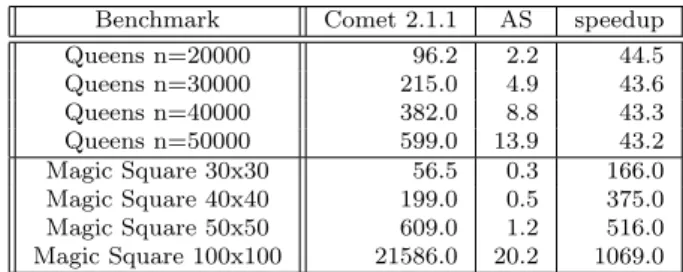
As regards other Local Search solvers, the 2003 version of AS was compet-itive with systems such as Comet for simple benchmarks (e.g., All-Interval or Magic-Square), according to timings given in [72]. As a very limited but more recent comparison, Table 1 compares the performance of AS with the Comet 2.1.1 system on a few basic CSPLib benchmarks provided in the distribution of Comet. Timings are in seconds and taken for both solvers on a PC with a Core2 Duo E7300 processor at 2.66 GHz, and are the average of 100 executions for AS and of 50 executions for Comet. Of course it should be noticed that Comet is a complete and very versatile system while Adaptive Search is just a C-based library, nevertheless we may point out that Adaptive Search is about two orders of magnitude faster than Comet, although better
performance could probably be achieved with a more refined Comet program (we used the programs in the standard distribution of Comet).
Benchmark Comet 2.1.1 AS speedup
Queens n=20000 96.2 2.2 44.5 Queens n=30000 215.0 4.9 43.6 Queens n=40000 382.0 8.8 43.3 Queens n=50000 599.0 13.9 43.2 Magic Square 30x30 56.5 0.3 166.0 Magic Square 40x40 199.0 0.5 375.0 Magic Square 50x50 609.0 1.2 516.0 Magic Square 100x100 21586.0 20.2 1069.0
Table 1: Execution times and speedups of Adaptive Search vs Comet
4 The Costas Arrays Problem
Let us describe a hard combinatorial problem originating from radar and sonar applications, the Costas Array Problem or CAP. This problem is challeng-ing for Constraint Programmchalleng-ing and propagation-based constraint solvers can only solve small instances of this problem [68] and therefore it is an interesting benchmark for parallelization.
4.1 Problem Description
A Costas array is an n × n grid containing n marks such that there is exactly one mark per row and per column and the n(n − 1)/2 vectors joining the marks are all different. We give here an example of Costas array of size 5. It is convenient to see the Costas Array Problem (CAP) as a permutation problem by consid-ering an array of n variables (V1, . . . , Vn) which forms
a permutation of {1, 2, . . . , n}. The Costas array in the figure opposite can thus be represented by the array [3, 4, 2, 1, 5].
4.1.1 Background
Historically, Costas arrays were developed in the 1960’s to compute a set of sonar and radar frequencies avoiding noise [27]. A very complete survey on Costas arrays can be found in [32]. The problem of finding a Costas array of size n is very complex since the required time grows exponentially with n. In the 1980’s, several algorithms were proposed to build a Costas array given n (methods to produce Costas arrays of order 24 to 29 can be found in [11, 34, 35,
66]), such as the Welch construction [39] and the Golomb construction [40], but these methods cannot built Costas arrays of size 32 and some higher non-prime sizes. Nowadays, after many decades of research, it remains unknown whether there exist any Costas arrays of size 32 or 33. Another difficult problem is to enumerate all Costas arrays for a given size. Using the Golomb and Welch constructions, Drakakis et al. present in [35] all Costas arrays for n = 29. They show that among the 29! permutations, there are only 164 Costas arrays, and 23 unique Costas arrays up to rotation and reflection. Indeed if the number of solutions for a given instance size n increases from n = 1 to n = 16, it then decreases from n = 17 onwards, reaching 164 for n = 29. Only a few solutions (and not all) are known for n = 30 and n = 31.
The Costas Array Problem has been proposed as a challenging combinato-rial problem by Kadioglu and Sellmann in [48]. They propose a Local Search metaheuristic, Dialectic Search, for constraint satisfaction and optimization, and show its performance for several problems. Clearly this problem is too difficult for propagation-based solvers, even for medium size instances (i.e., with n around 18 − 20). Let us finally note that we do not sustain that using Local Search is better than constructive methods in order to solve the CAP: rather, we consider the CAP as a very good benchmark for testing Local Search and constraint-based systems and to investigate how they scale up for large instances and parallel execution.
Rickard and Healy [65] studied a stochastic search method for CAP and concluded that such methods are unlikely to succeed for n > 26. Although their conclusion is true for their stochastic method, it cannot be extended to all stochastic searches: Their method uses a na¨ıve restart policy which is too basic, since they trigger a restart as soon as they find a plateau. Thus to find a solution, their algorithm must perform a perfect run decreasing the global cost at each iteration. However such runs are very unlikely for problems such as CAP where a tiny set of solutions is stranded amidst a huge search space. They also used an approximation of the Hamming distance between configurations in order to guide the search, which they admit not to be a very good indicator. In the same paper, the authors studied the distribution of solutions in the search space and showed that clusters of solutions tend to spread out from n > 17, which supports our finding that an independent multi-walk approach reaches linear speedup for high values of n, as presented in Section 5.
4.1.2 Basic Model
The CAP can be modeled as a permutation problem by considering an array of n variables V = (V1, . . . , Vn) which forms a permutation of {1, 2, . . . , n},
i.e., with an implicit all-different constraint over Vi. A variable Viis equal
to j iff there is a mark at column i and row j. To take into account constraints on vectors between marks (which must be different) it is convenient to use the so-called difference triangle [33].
This triangle contains n − 1 rows, each row corresponding to a distance d. The dth row of the triangle is of size n−d and contains the differences between any two marks at a distance d, i.e., the values Vi+d− Vifor all i = 1, . . . , n − d.
Ensuring that all vectors are different comes down to ensure the triangle contains no repeated values on any given row (i.e., all-different constraint on each row). Below is the difference triangle for the Costas array given as example in Section 4, which corresponds to the permutation V = (3, 4, 2, 1, 5) if we order columns and rows from the bottom left corner:
3 4 2 1 5
d = 1 1 -2 -1 4
d = 2 -1 -3 3
d = 3 -2 1
d = 4 2
In AS, the way to define a constraint is done via error functions. At each new configuration, the difference triangle is checked to compute the global cost and the cost of each variable Vi. Each row d of the triangle is checked one by
one. Inside a row d, if a pair (Vi, Vi+d) presents a difference which has been
already encountered in the row, the error is reported as follows: increment the global cost and the cost of both variables Vi and Vi+d by ERR(d) (a strictly
positive function). For a basic model we can use ERR(d) = 1 (to simply count the number of errors). Obviously a solution is found when the global cost equals 0. Otherwise AS selects the variable with the highest total error and tries to improve it.
4.1.3 Optimized Model
In the basic model, the function ERR(d) can be a constant (e.g., ERR(d) = 1) but a better function is ERR(d) = n2− d2 which “penalizes” more errors
occurring in the first rows (those containing more differences). The use of this function instead of ERR(d) = 1 improves the computation time (around 17%). Moreover, a remark from Chang [21] makes it possible to focus only on distances d ≤ b(n − 1)/2c. In our example, it is only necessary to check the two first rows of the triangle (i.e., d = 1 and d = 2). This represents a further gain in computation time (around 30%).
Another source of optimization concerns the reset phase. Recall that AS maintains a Tabu list to avoid to be trapped in local minima and, when too many variables become Tabu, the current configuration is perturbed to escape the current local minimum. We found that good results can be obtained with the following parameters: as soon as one variable is marked Tabu, reset 5% of the variables. Whereas this default behavior of AS is general enough to escape any local minimum, it sometimes “breaks” some important parts of the current configuration (but conversely, if we want to preserve too many variables, we can be trapped in the local minimum). AS allows the user to define his own reset procedure: when a reset is needed, this procedure is called to propose a pertinent alternative configuration. Our customized reset procedure tries 3 different perturbations from the current configuration:
1. Select the most erroneous variable Vm. Consider each sub-array starting
or ending by Vmand shift it (circularly) from 1 cell to the left and to the
right.
2. Add a constant “circularly” (i.e., modulo n to maintain the permutation) to each variable. The current implementation tries the 4 following con-stants: 1, 2, n − 2, n − 3 (but middle values n/2, n/2 − 1, n/2 + 1 revealed themselves to be also pertinent).
3. Left-shift from 1 cell the sub-array from the beginning to a (randomly cho-sen) erroneous variable different from Vm. In the current implementation
we test at most 3 erroneous variables.
All perturbations are considered one by one in order to find a perturbation able to escape the local minimum. For this detection, the global cost of the perturbation is compared to the global cost of the current configuration (ie. the configuration of the local minimum). Thus, as soon as the global cost of a perturbation is strictly inferior to the current global cost, the local minimum is considered as escaped and AS continues with this (perturbed) configuration. On average, this works in 32% of the cases (independently from n). Other-wise, all perturbations are tested exhaustively and the best (i.e., whose global cost is minimal, ties being broken randomly) is selected. This dedicated reset procedure provides a speedup factor of about 3.7 and is thus very effective.
4.2 Performance of Sequential Execution
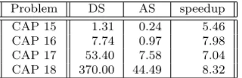
In [48], Kadioglu and Sellmann propose a novel and interesting Local Search metaheuristic called Dialectic Search (DS). Beyond classical CSP benchmarks, they show that their metaheuristic performs well on the Costas Array Problem and compare DS with a tabu search algorithm using the quadratic neighbor-hood implemented in Comet. The comparison was done for instances 13 to 18 and revealed that DS is between 2 and 3 times faster than Comet on Costas Array Problem. It is thus very interesting to compare our AS implementation with DS. Table 2 compares the results from [48] to the performance of AS on the same machine, a now outdated Pentium-III 733 MHz. Timings are in seconds and represent the average of 100 executions.
Problem DS AS speedup
CAP 15 1.31 0.24 5.46
CAP 16 7.74 0.97 7.98
CAP 17 53.40 7.58 7.04
CAP 18 370.00 44.49 8.32
Table 2: Execution times and speedups of Adaptive Search vs Dialectic Search
As the paper on DS does not provide any data other than execution time, we are unable to compare the number of iterations, local minima, etc. This
table clearly shows that AS outperforms DS on the Costas Array Problem: for small instances AS is five times faster but the speedup seems to grow with the size of the problem, reaching a factor 8.3 for n = 18.
Let us also remark that [48] also compares DS with the first (2001) version of AS [25] on Magic-Square with instances from 20x20 to 50x50, show-ing that both methods have similar results. However when usshow-ing the timshow-ings from [26], the second (2003) version of Adaptive Search is about 15 to 40 times faster than Dialectic Search on the same reference machine.
Following a CP model by Barry O’Sullivan, the Costas Array Problem has also been used as a benchmark in the Constraint Programming community, in particular in the MiniZinc challenge2. However, if solvers such as Gecode or the propagation-based engine of Comet can solve small instances up to CAP 18 in a few tens of seconds, medium size instances become clearly difficult and larger size instances are out of reach. For instance a CP Comet program3 needs more than 6 hours to solve CAP 19, while AS finds a solution in under one minute (on the same machine). A Gecode program4 will be a bit faster
but still needs more than 3 hours to solve CAP 19 (on the same machine). Simonis [68] reports on the performance of an improved model with refined propagation, which takes one minute to solve CAP 18 and a bit less than on hour to solve CAP 19 (on an unspecified machine).
5 Independent Multi-Walks
The independent multi-walk scheme consists of simultaneously running an instance of the algorithm under consideration on each core, without any com-munication during the search except at the very end: the first process reaching a solution sends an order to the others to stop their run and quit. Some non-blocking tests are involved every c iteration to check whether there is a message indicating that some other process has found a solution, in which case the cur-rent process terminates properly. Note however that several processes can find a solution “at the same time”, i.e., during the same c-block of iterations. Thus, those processes send their statistics (among which the execution time) to the process 0 which will then determine which one was actually the fastest.
The parallelization of the Adaptive Search method was done with two different implementations of the MPI standard, depending on the machine: OpenMPI on HA8000 and Grid’5000, and an extension of MPICH2 on JU-GENE.
Four testbeds were used to perform our experiments:
– HA8000, the Hitachi supercomputer of the University of Tokyo with a total number of 15,232 cores. This machine is composed of 952 nodes, each of which is composed of 4 AMD Opteron 8356 (Quad core, 2.3GHz, 512KB 2 http://www.g12.csse.unimelb.edu.au/minizinc/challenge2011/
3 written by Laurent Michel, personal communication. 4 http://www.hakank.org/gecode/costas_array.cpp
of L2-cache/core and 2MB of L3-cache/CPU, bus frequency 1000MHz) with 32GB of memory. Nodes are interconnected with a Myri10G net-work with a full bisection connection, attaining 5GB/sec in both directions. HA8000 has achieved a peak performance of 140Tflops, but we only had access to a subset of its nodes as users may only use a maximum of 64 nodes (1,024 cores) in normal service. HA8000 is running the RedHat Enterprise Linux distribution (RedHat 5).
– Grid5000 [17], the French national Grid for the research, which contains 8,596 cores deployed on 11 sites distributed in France. We used two subsets of the computing resources of the Sophia-Antipolis node: Suno, composed of 45 Dell PowerEdge R410 with 2 CPUs each (Intel Xeon E5520, Quad-core, 2.26GHz, 8MB of L2-cache/Quad-core, bus frequency at 1060MHz), thus a total of 360 cores with 32GB of memory, and Helios, composed of 56 Sun Fire X4100 with 2 CPUs each (AMD Opteron 275, Dual-core, 2.2GHz, 1MB of L2-cache/core, bus frequency at 400MHz), thus a total of 224 cores, with an access to 4GB of memory. Peak performance are 985GFlops for Helios and 3.25TFlops for Suno.
– JUGENE, the IBM Bluegene/P supercomputer at the J¨ulich Supercom-puting Centre in Germany. JUGENE is composed of 73,728 nodes with 4 CPUs each, bringing a total of 294,912 cores available. CPUs used by the Bluegene/P are 32-bit Power PC 450 CPUs (Mono-core, 850MHz, 8MB of L3-cache) with 2GB of memory. Compute nodes are linked through a 3D torus network with a theoretical bandwidth of 5.1GB/s. The overall peak performance reaches 1PFlops. JUGENE is running a SUSE Linux Enterprise distribution (SLES 10).
Notice also that despite our account on HA8000 allowing us to use up to 1,024 cores, the largest part of the experiments on this machine were carried out right after the March 11, 2011 earthquake in Japan, where electricity consumption restrictions allowed us to use only 256 cores for at most one hour.
5.1 Performance on Classical CSP Benchmarks
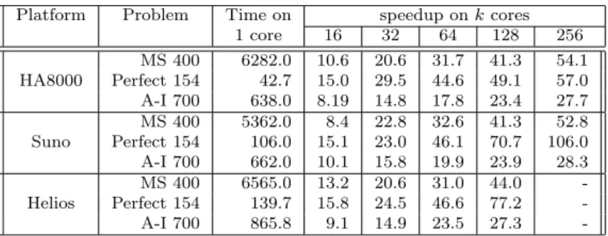
Parallel performance of a multi-walk version of AS are detailed in [19], which reports about executions up to 256 cores on HA8000 and on the Grid’5000 plat-form. Table 3 summarizes these results, considering the All-Interval Series (prob007 in CSPLib), the Perfect-Square placement problem (prob009 in CSPLib), and the Magic-Square problem (prob019 in CSPLib). The same code has been ported and executed on the different machines, timings are given in seconds and are the average of 50 runs, except for MS 400 on HA8000 where it is the average of 20 runs.
We run experiments on Magic-Square and All-Interval where the in-stance size n is respectively 400 and 700. Notice that an inin-stance for Perfect-Square cannot be encoded by a number only, since it consists of a set of squares of different size. Then we run our experiments on Perfect-Square
on the instance number 154 from CSPLib, known to be an instance of medium difficulty [12].
Platform Problem Time on speedup on k cores
1 core 16 32 64 128 256 HA8000 MS 400 6282.0 10.6 20.6 31.7 41.3 54.1 Perfect 154 42.7 15.0 29.5 44.6 49.1 57.0 A-I 700 638.0 8.19 14.8 17.8 23.4 27.7 Suno MS 400 5362.0 8.4 22.8 32.6 41.3 52.8 Perfect 154 106.0 15.1 23.0 46.1 70.7 106.0 A-I 700 662.0 10.1 15.8 19.9 23.9 28.3 Helios MS 400 6565.0 13.2 20.6 31.0 44.0 -Perfect 154 139.7 15.8 24.5 46.6 77.2 -A-I 700 865.8 9.1 14.9 23.5 27.3
-Table 3: Speedups on HA8000, Suno and Helios
We can observe that speedups are more or less equivalent on the three testbeds. Only in the case of Perfect-Square are the results significantly different for 128 and 256 cores. In those cases Grid’5000 has much better speedups than on HA8000. This is certainly because execution time is getting too small (less than one second) and therefore some other aspects interfere (OS background processes, system calls, . . .). Indeed, other explanations do not match: the cache memory size is not involved here since Helios and Suno nodes have the same behavior despite their different cache size, and there are few differences between cache sizes of HA8000 and Grid’5000 Helios nodes. Besides, the executable sizes are not involved either since each executable is just about 50KB on all architectures.
As we can see from the results we obtained, the parallelization of the method is effective on both the HA8000 and the Grid’5000 platforms, achiev-ing speedups of about 30 with 64 cores, 40 with 128 cores and more than 50 with 256 cores. Of course speedups depend on the benchmarks and here, the bigger the benchmark, the better the speedup. One can observe the stabiliza-tion point is not yet obtained for 256 cores, even if speedups do not increase as fast as the number of cores, i.e., are getting further away from linear speedup. As these experiments show that every speedup curve tends to flatten at some point, it suggests that there might be some sequential aspect with Lo-cal Search methods (or at least with AS) for those problems and that the improvement given by the multi-start aspect might reach some limit when in-creasing the number of parallel cores. This aspect of course depends on the energy landscape generated by the cost function. Moreover, this might be the-oretically explained by the fact that, as we use structured problem instances and not random instances, solutions may be not uniformly distributed in the search space but are regrouped in clusters, as was shown for solutions of the SAT problems near the phase transition in [51]. We will however see in the following section that there exist other problems like CAP for which linear speedups can be achieved even far beyond 256 cores.
5.2 Performance on the Costas Array Problem
We now present results of the parallel experiments for CAP. The following tables detail the execution times on HA8000 (Table 4), Grid’5000 (on Suno in Table 5, results on Helios are similar), and JUGENE (Table 7).
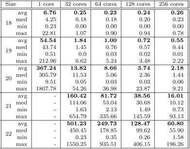
Each timing of the average, median, time and maximal times are computed from 50 runs of each benchmark, and given in seconds. Table 7 also contains the population standard deviation. We can see that with more cores, the maximal time decreases quite a lot and thus the runtime variation amplitude (i.e., the difference between minimal and maximal times) decreases drastically. More-over the median time is always below the average time, meaning we have fast runs more often than slow ones. Also, the median time presents a speedup at least as good as the average time: for instance for n = 20 on HA8000, the speedup w.r.t sequential time that is achieved using 256 cores is 170 for the average time and 210 for the median time.
Interestingly, one can observe that for large instances of CAP on JUGENE (Table 7), the value of the standard deviation is close to the mean value. This could be explained by the fact that the runtime distribution for a large instance of CAP is very close to an exponential distribution, cf. Figure 2 and Figure 4 in Section 5.3 for graphical examples, or see [70] for a detailed statistical analysis of the runtime distributions and their approximations by probability distributions. Indeed, it is a well-known property of the exponential distribution that the mean and standard deviation are equal. Also observe that having the median value smaller than the mean value is again a property of exponential distributions.
Size 1 core 32 cores 64 cores 128 cores 256 cores
18 avg 6.76 0.25 0.23 0.24 0.26 med 4.25 0.18 0.18 0.20 0.23 min 0.23 0.00 0.00 0.00 0.00 max 22.81 1.07 0.90 0.94 0.78 19 avg 54.54 1.84 1.00 0.72 0.55 med 43.74 1.45 0.76 0.57 0.44 min 0.51 0.0 0.03 0.02 0.01 max 212.96 6.62 5.24 3.48 2.22 20 avg 367.24 13.82 8.66 3.74 2.18 med 305.79 11.53 5.06 2.36 1.44 min 9.51 0.05 0.03 0.03 0.06 max 1807.78 54.26 36.98 23.87 9.21 21 avg - 160.42 81.72 38.56 16.01 med - 114.06 53.04 30.68 10.12 min - 1.63 2.13 1.49 0.73 max - 654.79 335.66 145.59 93.13 22 avg - 501.23 249.73 128.47 60.80 med - 450.45 178.85 99.62 55.90 min - 0.23 0.35 0.26 1.58 max - 1550.25 935.51 406.15 196.26
Size 1 core 32 cores 64 cores 128 cores 256 cores 18 avg 5.28 0.16 0.083 0.056 0.038 med 0.11 0.07 0.04 0.03 min 0.01 0.00 0.00 0.00 0.00 max 20.73 0.64 0.34 0.19 0.13 19 avg 49.5 1.37 0.59 0.41 0.219 med 1.09 0.38 0.33 0.155 min 0.67 0.02 0.01 0.00 0.02 max 279 9.41 2.74 1.82 1.12 20 avg 372 12.2 5.86 2.67 1.79 med 10.6 4.63 2.01 1.16 min 4.45 0.14 0.07 0.00 0.01 max 1456.00 50.60 26.00 19.20 8.50 21 avg 3743 171 51.4 34.9 17.2 med 108.00 38.50 21.80 10.80 min 265.00 5.56 0.24 0.27 1.05 max 10955.00 893.00 235 173 63.30 22 avg - 731 381 200 103 med - 428.00 286.00 135.00 69.50 min - 24.70 13.10 5.23 2.17 max - 6357.00 1482.00 656.00 451.00
Table 5: Execution times (in sec.) for CAP on Grid’5000 (Suno)
Table 6 shows in a concise manner the speedups obtained with respect to sequential execution on HA8000 and Grid’5000 for small and medium in-stances, i.e., 18 ≤ n ≤ 20. For small instances (n = 18), since computation times of parallel executions on many cores are below 0.5 second, they are maybe not significant because of interactions with operating system opera-tions. For medium instances (n = 19 and n = 20) speedup are close to linear, and we reach a speedup of 226 w.r.t. sequential execution for n = 19 on Suno with 256 cores.
Platform Problem Time on speedup on k cores
1 core 32 64 128 256 HA8000 CAP 18 6.76 27.00 29.40 28.20 26.00 CAP 19 54.54 29.60 54.50 75.70 99.20 CAP 20 367.20 26.60 42.40 98.20 168.00 Suno CAP 18 5.28 33.00 63.60 94.30 139.00 CAP 19 49.50 36.10 83.90 121.00 226.00 CAP 20 372.00 30.50 63.50 139.00 208.00 Helios CAP 18 8.16 34.00 74.20 136.00 -CAP 19 52.00 22.60 59.80 130.00 -CAP 20 444.00 31.00 58.20 98.20
-Table 6: Speedups for small and medium instances of CAP
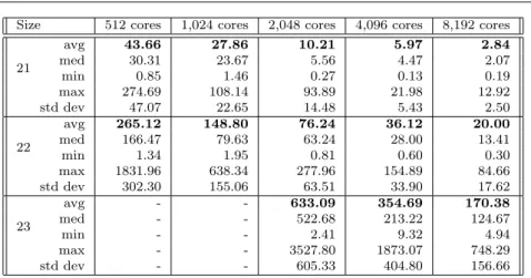
Table 7 shows the results on JUGENE for larger instances (n = 21, n = 22 and n = 23) and we present in a concise manner the speedups for the large instances in Table 8. Reference time for speedups are not sequential executions since it
Size 512 cores 1,024 cores 2,048 cores 4,096 cores 8,192 cores 21 avg 43.66 27.86 10.21 5.97 2.84 med 30.31 23.67 5.56 4.47 2.07 min 0.85 1.46 0.27 0.13 0.19 max 274.69 108.14 93.89 21.98 12.92 std dev 47.07 22.65 14.48 5.43 2.50 22 avg 265.12 148.80 76.24 36.12 20.00 med 166.47 79.63 63.24 28.00 13.41 min 1.34 1.95 0.81 0.60 0.30 max 1831.96 638.34 277.96 154.89 84.66 std dev 302.30 155.06 63.51 33.90 17.62 23 avg - - 633.09 354.69 170.38 med - - 522.68 213.22 124.67 min - - 2.41 9.32 4.94 max - - 3527.80 1873.07 748.29 std dev - - 605.33 404.80 156.66
Table 7: Execution times (in sec.) for CAP on JUGENE
becomes prohibitive (e.g., more than one hour for CAP21). Thus behaviors on all three platforms are similar and exhibit ideal speedups, i.e., linear speedups w.r.t. the base reference times.
Platform Problem Reference time speedup on k×reference cores
(#cores) k=2 (#cores) k=4 (#cores) k=8 (#cores)
HA8000 CAP 21 160.40 (32) 1.96 (64) 4.16 (128) 10.00 (256) CAP 22 501.20 (32) 2.01 (64) 3.90 (128) 8.24 (256) Suno CAP 21 171 (32) 3.32 (64) 4.90 (128) 9.94 (256) CAP 22 731.00 (32) 1.92 (64) 3.66 (128) 7.09 (256) Helios CAP 21 153.00 (32) 1.51 (64) 4.17 (128) -CAP 22 1218.00 (32) 2.34 (64) 5.53 (128) -JUGENE CAP 21 27.86 (1,024) 2.78 (2,048) 4.66 (4,096) 9.80 (8,192) CAP 22 148.80 (1,024) 1.95 (2,048) 4.11 (4,096) 7.44 (8,192) CAP 23 633.09 (2,048) 1.78 (4,096) 3.71 (8,192)
-Table 8: Speedups for large instances of CAP
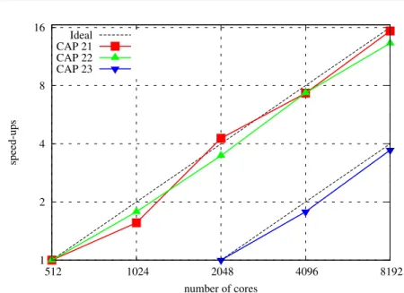
For n = 21 on Suno we have a 218 times speedup on 256 cores w.r.t. sequential execution. Concerning n = 22, as sequential computation takes many hours, we limit our experiments on all machines to executions on 32 cores and above. Therefore we will only give timings from 32 to 256 cores on HA8000 and Grid’ 5000 machines. On JUGENE, we were able to run experiments from 512 to 8,192 cores. This is graphically depicted with Figure 1 on a log-log scale. We can see that on all platforms, execution times are halved when the number of cores is doubled, thus achieving ideal or nearly ideal speedup. To the best of our knowledge, this is the first result on large-scale parallelism for CSP which achieves linear speedups over thousands of cores.
1 2 4 8 16 512 1024 2048 4096 8192 speed-ups number of cores Ideal CAP 21 CAP 22 CAP 23
Fig. 1: Speedups for CAP 21/22/23 on JUGENE
5.3 A More In-Depth Analysis
Since [75, 74], it is believed that combinatorial problems can enjoy a linear speedup when implemented in parallel by independent multi-walks. However this has been proven only under the assumption that the probability of finding a solution in a given time t follows an exponential law, that is, if the runtime behavior follows an exponential distribution (non-shifted). This behavior has been conjectured to be the case for Local Search solvers for the SAT problem in [44, 45], and shown experimentally for the GRASP metaheuristics on some combinatorial problems [2], but it is not always the case for constraint-based Local Search on structured problems. Indeed, [70] shows that the runtime dis-tribution can be exponential (e.g., Costas Array) but also sometimes log-normal (e.g., Magic-Square) or shifted exponential (e.g., All-Interval), in which cases the parallel speedup cannot be linear and the parallel speedup is asymptotically bounded. As mentioned earlier, a (pure) exponential runtime distribution may lead to a linear parallel speedup in theory, while a shifted exponential or lognormal will not.
The classical explanation for an exponential runtime behavior is the fact that the solutions are uniformly distributed in the search space, (and not regrouped in solution clusters [51]) and that the random search algorithm is able to sample the search space in a uniform manner. For the CAP instances, we could thus explain these linear speedups due to the good distribution of solutions over the search space for n > 17 as shown in [65] (although the number of solutions decreases beyond n = 17) and the fact that AS is able to diversify correctly.
Let us now look more precisely at the experimental runtime behavior of CAP instances and detail how it follows an exponential runtime distribution. Up to now we focused on the average execution time in order to measure the performance of the method, but a more detailed analysis could be done by looking at the runtime distribution. In [3, 64], a method is introduced to represent and compare execution times of stochastic optimization methods by using so-called time-to-target plots, in which the probability of having found a solution as a function of the elapsed time is measured. The basic idea is to fix a given value (target) to the objective function to optimize and to deter-mine the probability to reach this value for a given runtime t (hence the name time-to-target). Thus for any combinatorial optimization algorithm and any given target value for the objective function, the time-to-target plot can be constructed from the runtime results of the algorithm, i.e., more precisely from the cumulative distribution of the runtime (considered as a random variable), which gives the probability to reach a target value in a time less or equal to t. Observe that, for the CSPs, the objective function to minimize is the number of violated constraints and thus the target value to achieve is obviously zero, meaning that a solution is found. It is then easy to check if runtime distribu-tions can be approximated by a (shifted) exponential distribution of the form: 1 − e−(x−µ)/λ, where µ is the shift and λ is the scale parameter. Figures 2
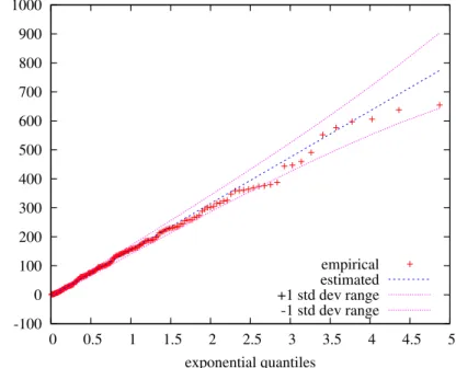
and 3 present the time-to-target plot for CAP 21 over 32 cores on HA8000 with its associated quantile-quantile plot obtained by plotting the quantiles of the data of the empirical distribution (red points) against the quantiles of the theoretical distribution, i.e., the exponential distribution (blue dashed line), see [3] for a detailed explanation of this construction. Approximations of the positive and negative standard deviation are shown in purple dashed line. If quantile-quantile data represented by red points remain between (or near) the two standard deviation lines, it means that our empirical runtime distribution can be approximated by a shifted exponential distribution. Such runtime dis-tribution plot and quantile-quantile plot are similar for CAP 21 over 64, 128 and 256 cores, and also for other large size instances.
Figure 4 presents together several time-to-target plots for CAP 21 in order to compare runtime distributions over 32, 64, 128 and 256 cores on HA8000. Points represent execution times (obtained over 200 runs) and lines correspond to the best approximation by an exponential distribution. It can be seen that the actual runtime distributions are very close to exponential distributions. Moreover, time-to-target plots also give a clear visual comparison between instances of the same method running with different numbers of cores. For instance we can see that there is an around 50% chance to find a solution within 100 seconds using 32 cores, but around 75%, 95% and 100% chance respectively with 64, 128 and 256 cores.
0 0.2 0.4 0.6 0.8 1 0 100 200 300 400 500 600 700 cumulative probability
time to target solution
empirical theoretical
Fig. 2: Time-to-Target plot for CAP 21 over 32 cores
-100 0 100 200 300 400 500 600 700 800 900 1000 0 0.5 1 1.5 2 2.5 3 3.5 4 4.5 5 measured times exponential quantiles empirical estimated +1 std dev range -1 std dev range
0 0.2 0.4 0.6 0.8 1 0 100 200 300 400 500 600 700 cumulative probability
time to target solution
32 cores 64 cores 128 cores 256 cores
Fig. 4: Time-to-Target plots for CAP 21 over 32, 64, 128 and 256 cores
6 Cooperative Multi-Walks
In order to take full advantage of the execution power of massively paral-lel machines, we have to seek a new way to further increase the benefit of parallelization, i.e., to try to reach linear speedups for problems which are sub-linear, such as Magic-Square or All-Interval. In the context of Local Search, we can consider a more complex parallel scheme, with communication between processes in order to reach better performance by favoring processes that seem to be closer to a solution (i.e., whose current global cost value is low) versus processes which are far away from it. So we aim at providing inter-process communication in order to exchange little information and let some processes decide to trigger a restart depending on the state of the others. This fits in the framework of dependent cooperative multi-walks. A good candidate for the information to exchange between processes is the value of the current cost of each process, as it is small in size (only one integer) and it is a heuristic which approximates the speed to reach a solution.
6.1 COST and ITER algorithms
The basic idea of the method with communicating Local Search processes is as follows:
– Every c iterations a process sends to other processes (for algorithm COST) the cost of its current best total configuration and (for algorithm ITER) also the number of iterations used to obtained it.
– Every c iterations each process also checks messages from other processes, and for each message with (for algorithm COST) a lower cost or (for algo-rithm ITER) a lower cost and a lower number of iterations, lower than its own – meaning it is further away from a solution from the metric perspec-tive – it can decide to stop its current computation and make a random restart. This will be done following a given probability p.
Note that communication is implemented with asynchronous sends and re-ceives. We use a log2(n) binary spanning tree to define node neighbours, in order to limit the aggregate communication requirements which could other-wise become very significant with a large number of processes: as it stands we have O(n) send-receive pairs. A process propagates the maximum of its own cost and the received cost values, by forwarding it to its neighbours.
Therefore the two key parameters are c, the number of iterations between messages and p, the probability to make a restart. The COST and ITER algo-rithms do not differ very much; intuitively, the ITER algorithm incorporates a more precise measurement (a process is considered better than another one if it has reached a better cost in a smaller number of iterations).
6.2 Experimental results
In order to investigate the behavior of the COST algorithm and of the ITER algorithm, we used the Helios cluster of Grid’5000, from 32 cores up to 128.
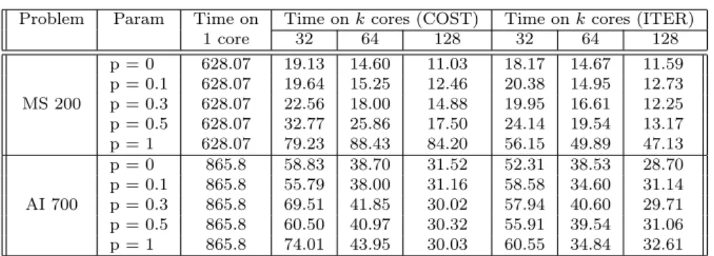
Table 9 presents the average on 50 runs of the execution time of the prob-lems Magic-Square 200 and All-Interval 700, from 32 to 128 cores, run-ning the COST and ITER algorithms with different values for the parameter p. Concerning the c parameter, it is clear that if c is too small the performance will decrease (too many restarts) and if it is too large then it will not have much influence on the computation. We found that the best trade-off is to adjust c according to the problem in order to have communication once or a few times per second, considering that we have an average sequential runtime of several hundreds of seconds. This will give c = 1000 for Magic-Square 200 and c = 100 for All-Interval 700. The overhead of communication is thus negligible when such value for c is chosen. Please note that a value p = 0 leads to the same behavior as the independent multi-walk algorithm (with no communication), since even if communication is performed, the received cost value is never considered and does not impact each process decision to restart. It thus makes it possible to compare the cooperative multi-walk algorithm with the previous independent multi-walk algorithm.
Let us firstly note that the COST and ITER algorithms do not differ much in their results. However ITER is better on Magic-Square, especially for higher values of p, which can be easily explained because it performs less
Problem Param Time on Time on k cores (COST) Time on k cores (ITER) 1 core 32 64 128 32 64 128 p = 0 628.07 19.13 14.60 11.03 18.17 14.67 11.59 p = 0.1 628.07 19.64 15.25 12.46 20.38 14.95 12.73 MS 200 p = 0.3 628.07 22.56 18.00 14.88 19.95 16.61 12.25 p = 0.5 628.07 32.77 25.86 17.50 24.14 19.54 13.17 p = 1 628.07 79.23 88.43 84.20 56.15 49.89 47.13 p = 0 865.8 58.83 38.70 31.52 52.31 38.53 28.70 p = 0.1 865.8 55.79 38.00 31.16 58.58 34.60 31.14 AI 700 p = 0.3 865.8 69.51 41.85 30.02 57.94 40.60 29.71 p = 0.5 865.8 60.50 40.97 30.32 55.91 39.54 31.06 p = 1 865.8 74.01 43.95 30.03 60.55 34.84 32.61
Table 9: Execution times with COST & ITER algorithms (in seconds)
restarts than COST and in this case performing restarts amounts to worse performance.
Secondly, the results are quite different depending on the problem: For Magic-Square, communication only slightly affects performance for a prob-ability of restarting p < 0.5. But when we monitored the number of restarts, we saw a sharp increase of this number related to the increasing value of p: there are almost no restarts for p < 0.5, but there is an average of 43 for p = 1. Thus, in this case, favoring a restart if another process has a better cost value does not improve the average execution time at all and indeed, it actually decreases performance w.r.t. the independent multi-walk scheme. For All-Interval, communication does not have much impact on performance nor on the number of resets/restarts which are on average between 4 and 5 (with a standard deviation of 5). Results are basically similar to those obtained with the independent multi-walk scheme.
It is thus difficult with these simple communication schemes to achieve better performance than the initial method with no communication. This can be explained by the fact that the metric used to indicate that one Local Search engine instance is better than another, which is in our case the current value of the cost function, is not very reliable to compare execution process between them, even if it shows to be efficient in the execution process itself. The value is an heuristic value and is thus not as reliable an information as would be, for instance, the value of the bound that could be communicated between processes in a parallel Branch & Bound algorithm.
Let us illustrate this problem with some data collected during experiments of parallel executions. Figure 5.a shows the evolution of the cost function of the current configurations examined on some processes within a 64-core exe-cution by the parallel Adaptive Search algorithm on the Magic-Square 400 benchmark, as computation is performed and the number of iterations grows. In this experiment, process 42 is the fastest to find an answer. Nonetheless it is clear that the two other processes are indeed decreasing the cost func-tion faster but either need a reset/restart (Process 9) or will continue with a low cost without reaching a solution (Process 49). This is maybe not very
Plot for Proc. 9 Plot for Proc. 0
Plot for Proc. 49 Plot for Proc. 1
Plot for Proc. 42 Plot for Proc. 10 0 2k 4k 6k 8k 10k 12k 14k 16k 18k Nb of iterations 0 2k 4k 6k 8k 10k 12k 14k 16k Nb of iterations 0 2k 4k 6k 8k 10k 12k 14k 16k Nb of iterations 0 500 1000 1500 2000 2500 3000 Nb of iterations 0 1000 2000 3000 4000 5000 6000 Nb of iterations 0 500 1000 1500 2000 2500 3000 3500 Nb of iterations C o st (x 10 ) Cost Cost Cost 700 600 500 400 300 200 100 0 700 600 500 400 300 200 100 0 700 600 500 400 300 200 6 5 4 3 2 1 0 8 C o st (x 10 ) 8 C o st (x 10 ) 8 6 5 4 3 2 1 0 7 6 5 4 3 2 1 0 7
a) Magic Square 400 b) All-Interval 700 Fig. 5: Evolution of costs
clear from Figure 5.a because the Y-axis (cost value) represents multiple of 108 and thus both process 42 and 49 seem to reach a cost value of zero, but
indeed only process 42 does so, after about 15000 iterations. Figure 5.b shows a similar experiment on the All-Interval 700 benchmark. Here the value of the cost function fluctuates even more, as every process needs a few resets. Process 10 is the fastest to reach a solution, but it is not clear to foresee it from the successive values of the cost of the configurations examined during the computation.
To conclude, it is important to note that the two (simple) algorithms with communication of the cost value that we have considered (COST & ITER algorithms) actually do not achieve better results than the independent multi-walk scheme. It is also interesting to link these results to the experiments described in [7] for parallel SAT with the Sparrow solver [10], the best local search SAT solver in the 2011 SAT competition. These experiments compare parallel algorithms with and without cooperation, although communication is performed in a different manner than the one proposed here: parallel processes communicate their configurations at each restart (restart is an important fea-ture for SAT local search) and the Prob NormalizedW heuristics [9] is used for aggregating those configurations and defining a good restart configuration, supposedly better than a random restart. This paper shows, in a different problem domain and with a different solver, that it is difficult to perform bet-ter than the independent multi-walk version, both in capacity solving (number of instance solved) and with respect to the PAR-10 metrics [46].
7 Conclusion and Future Work
We presented a parallel implementation of a constraint-based Local Search algorithm, the Adaptive Search method with both independent and cooper-ative multi-walk variants. Experiments have been carried out using CSPLib benchmarks as well as a real-life problem, the Costas Array Problem, which has applications in telecommunications. Performance evaluation on four dif-ferent parallel architectures (two supercomputers and two clusters of a Grid platform) shows that the method achieves speedups better than 50 with 256 cores on classical CSP benchmarks, which is good but far from linear speedup. More interesting is the Costas Array Problem, for which execution times are halved when the number of cores is doubled and thus linear speedups have been observed up to 8,192 cores. We presented in this paper a novel model and solv-ing process for the Costas Array Problem in the Adaptive Search framework, which is very efficient sequentially (nearly an order of magnitude faster than previous approaches) and which scales very well in parallel. It seems therefore that the simple paradigm of independent multi-walks is a good candidate for taking advantage of the computing power of massively parallel machines for hard combinatorial problems. Up to our knowledge, this is the first result on large-scale parallelism for CSP or Local Search reaching linear speedups over thousands of cores.
We also made an attempt to extend the independent multi-walk parallel scheme by using simple cooperation and communication between processes. The key idea is to force processes which are further away from optimal solutions (i.e., for which the best value obtained of the objective function obtained so far is worse than that of the best of the parallel processes) to restart their search trajectory. Although modulated by a probability parameter aimed at controlling the restarts, these schemes force too many processes to restart too soon, i.e., to abandon otherwise possibly promising search trajectories, and
thus cannot achieve better performance than the basic independent multi-walk scheme (on average).
Further work and experiments are thus still needed to define a parallel method with inter-process communication that could outperform the initial basic independent multi-walk method. Our current work is focusing on a com-munication mechanism which implies 1) a number of restarts as low as pos-sible if we want the parallel execution to benefit from the parallelization of the Adaptive Search algorithm; 2) a reduction in the sequential aspect of the resolution by re-using some common computations or by recording pre-vious interesting crossroads during the resolution, from which a restart can be operated; 3) sharing such information with asynchronous but coordinated inter-process transfers.
Acknowledgements We acknowledge that some results in this paper have been achieved using the PRACE Research Infrastructure resource JUGENE based in Germany at the J¨ulich Supercomputing Centre, while some others were carried out using the Grid’5000 experimental testbed, being developed under the INRIA ALADDIN development action with support from CNRS, RENATER and several Universities as well as other funding bodies.
References
1. Aida, K., Osumi, T.: A case study in running a parallel branch and bound application on the grid. In: SAINT ’05: Proceedings of the 2005 Symposium on Applications and the Internet, pp. 164–173. IEEE Computer Society, Washington, DC, USA (2005) 2. Aiex, R., Resende, M., Ribeiro, C.: Probability distribution of solution time in GRASP:
An experimental investigation. Journal of Heuristics 8(3), 343–373 (2002)
3. Aiex, R., Resende, M., Ribeiro, C.: TTT plots: a Perl program to create time-to-target plots. Optimization Letters 1, 355–366 (2007)
4. Alava, M., Ardelius, J., Aurell, E., Kaski, P., Orponen, P., Krishnamurthy, S., Seitz, S.: Circumspect descent prevails in solving random constraint satisfaction problems. PNAS 105(40), 15,253–15,257 (2007)
5. Alba, E.: Special issue on new advances on parallel meta-heuristics for complex prob-lems. Journal of Heuristics 10(3), 239–380 (2004)
6. Amdahl, G.: Validity of the single processor approach to achieving large scale computing capabilities. In: proceedings of AFIPS’67, spring joint computer conference, pp. 483– 485. ACM Press, Atlantic City, New Jersey (1967). URL http://doi.acm.org/10.1145/ 1465482.1465560
7. Arbelaez, A., Codognet, P.: Massively parallel local search for SAT. In: proceedings of ICTAI’2012, IEEE 24th International Conference on Tools with Artificial Intelligence, pp. 57–64. IEEE Press (2012)
8. Arbelaez, A., Codognet, P.: From sequential to parallel local search for SAT. In: M. Mid-dendorf, C. Blum (eds.) proceedings of EvoCOP13, 13th European Conference on Evo-lutionary Computation in Combinatorial Optimization, Lecture Notes in Computer Sci-ence, vol. 7832, pp. 157–168. Springer Verlag (2013)
9. Arbelaez, A., Hamadi, Y.: Improving Parallel Local Search for SAT. In: C. Coelo (ed.) Learning and Intelligent Optimization, Fifth International Conference, LION 2011. LNCS, Rome, Italy (2011)
10. Balint, A., Fr¨ohlich, A., Tompkins, D., Hoos, H.: Sparrow2011. In: Solver Description Booklet, SAT competition 2011 (2011)
11. Beard, J., Russo, J., Erickson, K., Monteleone, M., Wright, M.: Costas array generation and search methodology. IEEE Transactions on Aerospace and Electronic Systems 43(2), 522–538 (2007)