Neurocomputing 70 (2006) 70–77
Combining an evolutionary algorithm with data mining
to solve a single-vehicle routing problem
H.G. Santos
, L.S. Ochi, E.H. Marinho, L.M.A. Drummond
Department of Computer Science, Universidade Federal Fluminense, Nitero´i, Brazil
Available online 22 August 2006
Abstract
The aim of this work is to present some alternatives to improve the performance of an evolutionary algorithm applied to the problem known as the oil collecting vehicle routing problem. Some proposals based on the insertion of local search and data mining (DM) modules in a genetic algorithm (GA) are presented. Four algorithms were developed: a GA, a GA with a local search procedure, a GA including a DM module and a GA including local search and DM. Experimental results demonstrate that the incorporation of DM and local search modules in GA can improve the solution quality produced by this method.
r2006 Elsevier B.V. All rights reserved.
Keywords:Evolutionary algorithms; Data mining; Vehicle routing
1. Introduction
Evolutionary algorithms and genetic algorithms (GA), its most popular representative, are part of the research area of artificial intelligence inspired by the natural evolution theory and genetics, known as evolutionary computation. Those algorithms try to simulate some aspects of Darwin’s natural selection and have been used in several areas to solve problems considered intractable (NP-complete and NP-hard). Although these methods provide a general tool for solving optimization problems, their traditional versions [26,11,15] do not demonstrate much efficiency in the resolution of high complexity combinatorial optimization (CO) problems. This deficiency has led researchers to propose new hybrid evolutionary algorithms (HEA) [8,24,5], sometimes named ‘‘memetic algorithms’’ ([20,21], which usually combine better con-structive algorithms, local search and specialized crossover operators. The outcome of these hybrid versions is generally better than independent versions of these algo-rithms. In this paper we propose an HEA for a routing problem which incorporates all features cited before plus an additional module of data mining (DM), which tries to
discover relevant patterns in the best solutions found so far, in order to guide the search process to promising regions of the search space. After presenting the problem, we describe a GA and afterwards, three improved versions: GA with local search, GA with DM and GA with DM and local search.
2. The oil collecting vehicle routing problem
Concerning oil exploitation, there is a class of onshore wells called artificial lift wells where the use of auxiliary methods for the elevation of fluids (oil and water) is necessary. In this case, a fixed system of beam pump is used when the well has a high productivity. Because oil is not a renewable product, the production of such wells will diminish until the utilization of equipment permanently allocated to them will become economically unfeasible. The exploitation of low productivity wells can be done by mobile equipment coupled to a truck. This vehicle has to perform daily tours visiting wells, starting and finishing at the oil treatment station (OTS), where separation of oil from water occurs. Usually the mobile collector is not able to visit all wells in a single day. In this context, arises the problem called oil collecting vehicle routing problem (OCVRP). In this problem, the objective is to collect the maximum amount of oil in a single day, starting and
www.elsevier.com/locate/neucom
0925-2312/$ - see front matterr2006 Elsevier B.V. All rights reserved. doi:10.1016/j.neucom.2006.07.008
finishing the route at OTS, respecting time constraints. The OCVRP can be considered as a generalization of the traveling salesman problem (TSP) which is classified as NP-hard. Thus, it is possibly harder to solve than the TSP. Formally, given a setW ¼ f1;. . .;ngof locations, where
location 1 represents OTS and all other locations represent wells, letpibe the estimated daily production of welli2W
(p1¼0), tij be the estimated time for traveling from
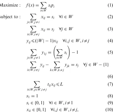
location i to location j and L the time limit for routes, the OCVRP can be formulated as the following mixed integer programming (MIP) problem:
Maximize: fðxÞ ¼ X
i2W
sipi ð1Þ
subject to:
X
j2W;jai
xij¼si 8i2W ð2Þ
X
i2W;iaj
xij¼sj 8j2W ð3Þ
yijpðjWj 1Þxij 8i;j2W;iaj ð4Þ
X
j2W;ja1
y1j¼ X
i2W
si
!
1 ð5Þ
X
i2W;iaj
yij X
k2W;kaj
yjk ¼sj 8j2W f1g
ð6Þ
X
i2W;j2W;iaj
tijxijpL ð7Þ
s1¼1 ð8Þ
si2 f0;1g 8i2W;ia1 ð9Þ
xij2 f0;1g 8i;j2W;iaj, ð10Þ
wheresiindicates if welliwill be visited, that is, whether it
is part of the route (si¼1) or not (si¼0) andxijindicates
whether arc (i;j) will be included on the route (xij¼1) or
not (xij¼0). Constraints (2) and (3) ensure that for active
wells, and only for these wells, there must be one input and one output arc included in the route. Constraints (4)–(6) are subtour-elimination constraints, where yij represents
the ‘‘flow’’ in arc ði;jÞ [22]. Constraint (7) prevents from exceeding the time limit, and constraint (8) ensures that OTS is included in the route.
Although for routing problems in general there are some recent successful applications of GAs [5,19,24], for problems similar to OCVRP, such as the traveling purchaser problem [25], the prize collecting problem [4]
and the orienteering problem[12], they are scarce[13].
3. Genetic algorithm
This section describes an overview of the GA proposed to solve the OCVRP. In order to represent a solution, we employ a direct representation, where each individual is coded by a variable size list of integer numbers, where genes correspond to wells pertaining to route coded by an individual. The last gene of each individual always
represents the oil treatment station, using 1 to code it. The position of a well in this list represents its order in the route. A sample individual is showed inFig. 1. In this case, the following route is represented: OTS well 16 well 34
- well 58 - well 44 - OTS. Note that the route always starts at OTS, in spite of the first gene not representing it. Throughout the text, we will denote individuals byindand
wellsðindÞwill denote the number of wells of individualind. Also, indi will denote the ith visited well (or OTS, for
indwellsðindÞþ1) andtimeðindÞ will denote the time needed to
perform the route encoded in ind. The fitness function is exactly the objective function presented in Section 2.
To generate the initial population, individuals are constructed using an iterative procedure, similar to the constructive phase of GRASP[7,29]. They are built taking into account a greedy criterion which is used to define which wells can be included in partial solutions. This criterion is based onpi=tjiratio, wherepiis the production
rate of the candidate welliandtjiis the time spent to travel
from the last well j included in the partial solution to the welli. Thus, at each iteration, a well is selected from a list that contains all wells not yet included in the solution, with
pi=tji ratio in the range ½rmin;rmax. Let r be the greatest
pi=tjiratio among all wells not yet included in the solution
and r be the smallest ratio among these same wells then
rmin¼raðrrÞandrmax¼r. Theaparameter should be
selected in the range [0,1], allowing the choice of the randomization degree of individual generation. This process is executed while the total time consumed on the route being constructed has not reached the time limit L. Once the addition of a given wellw2W produces a partial route with an associated time greater or equal than the time limit (not including the time to return to OTS), the reparation procedure is started.
The reparation procedure transforms an incomplete, infeasible solution, into a complete, feasible one, in the following way: in order to turn the OTS inclusion possible, this procedure removes, iteratively, the last well in the route until the solution including OTS satisfies the time limit constraint.
Our GA uses a genetic operator different from tradi-tional crossover operators. A new individual (offspring) is generated from np solutions (parents) of the current population, where np varies from one up to the size of the population. Each parent solution is chosen by a tournament procedure that selects the fittest individual from a set of k individuals randomly selected from the population.
The crossover operator proposed here combines infor-mation from parent solutions and the heuristic criterion employed in the constructive phase, as follows: during each iteration of offspring generation, a well is chosen to take
part in the route. This well is randomly chosen from a list of remaining wells taking into account a probability distribution that favors the addition of wells with the highest gi¼ ð1þzjiÞ ðpi=tjiÞ, where zji is the frequency
which welli(candidate well) is the successor of wellj(last well added to the partial solution) in parent solutions. The probability of choosing a given well is proportional to the position of this well in a list sorted by non-ascending order of the greedy criteriongi, as suggested in[6]. In this work,
polynomial distribution probability was chosen. This process is executed while the total time consumed on the route being constructed has not reached the time limit. It is important to note that our crossover operator does not rely only on information from parent solutions, allowing the occurrence of offsprings with genetic code not available on parents. Thus, there is no need of incorporating a mutation operator. During the evolutionary process, the population remains at a fixed size, i.e., the insertion of b new individuals substitutes the b worst individuals in the population.
3.1. GA with local search
Local search is a post-optimization procedure that allows a systematic search in a solution space by using a neighborhood structure [17]. In this work two neighbor-hood structures were used, aimed at increasing the amount of collected oil for a feasible solution for the problem (base solution).
In both neighborhoods, whose pseudo-codes are shown in Figs. 2 and 3, a set Uof wells not yet included in the current solution is maintained. The first neighborhood—
N1 (procedure Insert), tries to add into the current
solution each well pertaining to setU, searching for the first possible position for insertion, from 0, before the first visited well, until wellsðindÞ, after the last one. In line 7,
insertionðind;u;kÞ represents the increase in time resulting from the insertion ofu in the route ofind, at positionk.
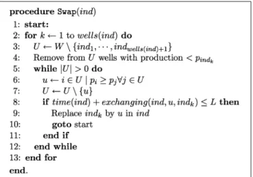
The second neighborhood—N2 (procedureSwap), tries
to exchange each well from the current solution with
another from set U. In line 8, exchanging(ind, u, indk)
represents the variation in time needed to perform the route encoded inindderived from the replacement of well
indk by well u in ind. First fit criterion is used in both
neighborhoods and the search in a given neighborhood is re-started whenever a better solution is found. Elements are accessed in the setUin non-increasing order. Local search operators are applied in newly created solutions from crossover operations and from the DM intensification procedure, explained in the following section. The prob-ability of applying local search in these individuals, with neighborhoodsN1 andN2 are controlled by parameters probN1 andprobN2.
3.2. GA with DM
With the aim of accelerating the occurrence of high quality solutions in the population, we propose the incorporation of a DM module in the GA. This module aims to discover patterns (subroutes) which are commonly found in the best solutions of the population. This approach significantly differs from current applications that combine GAs and DM because, until now, most of the efforts deal with the development of GAs as optimization methods to solve DM problems [14,10], such as the discovery of association, classification and clustering rules, which is not our case. The process starts with the creation of an elite set of solutions (ES), which will keep thesbest solutions generated in the search process. Initially, the first
s solutions generated are inserted in the ES. Afterwards, this set is updated whenever a solution which is better than the worst solution in ES and different from all others ES solutions is generated. The ES will be the database in which we will try to discover relevant patterns. In order to do this, we implemented an Apriori like algorithm [1,2], which discovers frequent contiguous sequences in the ES. Although there are very efficient algorithms for mining sequential patterns, we chose to implement a simpler one, for two reasons: at first, our ES size will be significantly
Fig. 2. Pseudo-code forInsert.
smaller than databases which are generally considered for DM (for this type of CO problem, good solutions are computationally expensive to produce); secondly, we focused on the specific problem of finding contiguous sequences, which is easier to solve than more general sequence pattern mining problems [9,23]. The algorithm receives the minimum support as an input parameter. This parameter is related to the size of ES and defines the minimun number of occurrences in ES that one sequence must have to be considered frequent. Thus, the algorithm will discover all sequences (subroutes in the ES) of all sizes
ðX1Þ, which satisfy the minimal support. For instance, a minimum support of 0.5, indicates that at least half of ES solutions must incorporate the considered sequence.
Once a set of frequent sequences is available, it is used to guide the construction of new individuals, in the following way: new individuals are built using a constructive procedure similar to the one used to build new solutions from crossover operations, except that no information of frequency in parent solutions is available ðzij¼0;8i;jÞ,
furthermore, whenever a well is selected to be added to the partial solution, a set of valid subroutes is built. This set contains only frequent sequences whose wells do not appear in the partial solution, starting with the selected well. If more than one subroute is found, we randomly choose from the available ones. The sequence chosen is incorporated in partial solution. Since time limit constraint can easily be violated through the addition of a sequence of
wells, the reparation operator presented in Section 3 is applied. If no valid subroute is found in DM results, only the selected well is added. Each time that the DM module is triggered, b new individuals are generated using data mining information. As in crossover operator, population remains at a fixed size.
Remark that the discovery of relevant patterns relies on having a good set of elite solutions. In the beginning of the search the average fitness of population continually increases, causing frequent changes in ES. Hence, data mining is only worth applying after some iterations have been processed. Also, after the first DM execution, newer ones must only occur if the ES was modified. The parameter m controls how often the DM module will be activated. On setting up this parameter, very small values shall not be used, in order to avoid premature convergence.
3.3. GA with DM and local search
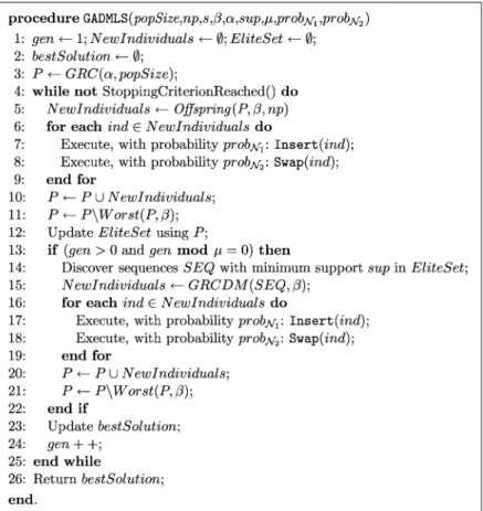
The application of DM can be used together with local search procedures, through the application of local search in new individuals from crossover operator and from DM procedure. This configures the most complete version of GA proposed here, named genetic algorithm with data mining and local search (GADMLS). The pseudo-code for this algorithm is presented in Fig. 4. Initial population is generated using the greedy randomized constructive (GRC) procedure (line 3), which was described in Section 3.
Function Offspring (line 5) indicates the application of crossover operator usingnpparent solutions from popula-tionP to generate each one of the b new individuals. To keep a fixed population size through generations,b worst individuals of population (function Worst) are removed wheneverbnew individuals are included. In the application of data mining (lines 14 and 15), b new individuals are generated using the discovered frequent sequencesSEQby
the GRCDM procedure GRC, whose functioning was
described in Section 3.2. The best solution of all genera-tions (with the highest value of fitness functionfðxÞ, where
x is the evaluated solution) is kept and returned by the algorithm. Simpler versions of this algorithm (GA without local search and/or DM) are just as the algorithm inFig. 4, except by the removal of modules of DM (lines 13–22) and/ or local search (calls toInsertandSwap).
3.4. Computational results
To the best of our knowledge no set of instances were made publicly available to the OCVRP. Thus, a set of
instances (Table 1) with different characteristics were generated. Instances incorporate distances from TSP-library problems[28]which can be found at[27]. For each TSP-library problem used, four problems were generated, with different well productions and different time limits. Time limits were defined in a way that no trivial solution was possible (including all wells): these values are always a fraction of the optimal tour length. The naming convention used for problems was the following: sourceTSP_ max-Prod_timeLimitF. Where sourceTSP is the name of the original TSP instance. Production of wells was randomly generated using uniform distribution in the interval
f1;. . .;maxProdg. Time limit for each instance is
time-LimitF percent of the optimal tour length from
TSP-Library. In Table 1, columns ‘‘rows’’, ‘‘columns’’ and ‘‘binaries’’ are related to the dimensions of the generated MIP problems: number of constraints, variables and binary variables, respectively.
Algorithms were coded in C and compiled with theGCC
3.3.4 compiler, using flag -O2. Running times were measured with thegetrusage function. Pseudo random
Table 1
Problem characteristics
P. Id. Problem name Rows Columns Binaries Execution time limit (s)
1 ulysses22_1000_40 529 945 483 5
2 ulysses22_1000_70 529 945 483 7
3 ulysses22_100000_40 529 945 483 4
4 ulysses22_100000_70 529 945 483 7
5 att48_1000_40 2401 4559 2303 9
6 att48_1000_70 2401 4559 2303 13
7 att48_100000_40 2401 4559 2303 9
8 att48_100000_70 2401 4559 2303 13
9 st70_1000_40 5041 9729 4899 16
10 st70_1000_70 5041 9729 4899 25
11 st70_100000_40 5041 9729 4899 16
12 st70_100000_70 5041 9729 4899 25
13 ch130_1000_40 17,161 33,669 16,899 57
14 ch130_1000_70 17,161 33,669 16,899 92
15 ch130_100000_40 17,161 33,669 16,899 59
16 ch130_100000_70 17,161 33,669 16,899 93
17 d198_1000_40 39,601 78,209 39,203 189
18 d198_1000_70 39,601 78,209 39,203 276
19 d198_100000_40 39,601 78,209 39,203 160
20 d198_100000_70 39,601 78,209 39,203 272
21 a280_1000_40 78,961 156,519 78,399 227
22 a280_1000_70 78,961 156,519 78,399 396
23 a280_100000_40 78,961 156,519 78,399 227
24 a280_100000_70 78,961 156,519 78,399 396
25 pr439_1000_40 193,600 385,002 192,720 809
26 pr439_1000_70 193,600 385,002 192,720 1401
27 pr439_100000_40 193,600 385,002 192,720 797
28 pr439_100000_70 193,600 385,002 192,720 1389
29 pcb442_1000_40 196,249 390,285 195,363 683
30 pcb442_1000_70 196,249 390,285 195,363 1126
31 pcb442_100000_40 196,249 390,285 195,363 697
32 pcb442_100000_70 196,249 390,285 195,363 1137
33 att532_1000_40 284,089 565,515 283,023 1359
34 att532_1000_70 284,089 565,515 283,023 2019
35 att532_100000_40 284,089 565,515 283,023 1356
numbers were generated using Mersenne twister generator
[18]. Experiments were executed in a microcomputer with an Athlon XP 1800+ processor and 512 Megabytes of RAM, running the Linux operating system, kernel 2.4.29. In this section the simplest algorithm will be referred as GA, while its composition with local search will be referred as GALS, the hybrid version with data mining will be referred as GADM and GADMLS indicates the version which includes local search and data mining.
In order to compare different versions of algorithms, we stipulated fixed time limits (stopping criterion in the algorithm of Fig. 4), for each instance. Execution time limits are proportional to instances dimensions, as follows: given a instance i, the allowed execution time tli is:
tli¼tcik, wheretciis the time needed to build a solution
using the constructive algorithm described in Section 3 and
k is a sufficiently large constant (20,000 in our experi-ments).
The following parameters were used in our GA:
Population size (popSize): 500. New individuals (b): 50. Number of parents (np): 50. Randomization degree (a): 0.5. Tournament individuals: 2.Versions with the DM module had the additional parameters:
Minimum support (minSup): 0.5. Elite set size: (s): 5. Mining interval: (m): 50.For versions with local search, all new solutions were transformed in local optima with respect to both neighbor-hoods, i.e.:probN1¼1:0 and probN2¼1:0.
In Table 2, we show the average solution value, with standard deviation, produced in 10 independent executions (different random seeds), for different versions of our
algorithms. Results in bold indicate the better average results. As can be seen, in 80% of problems, the outcome of version with DM (GADM) is better than the outcome of version without this module (GA). In any case, the hybrid GA with DM and local search obtained, overall, the best results: it produced the best average solution in 22 out of the 36 problem instances.
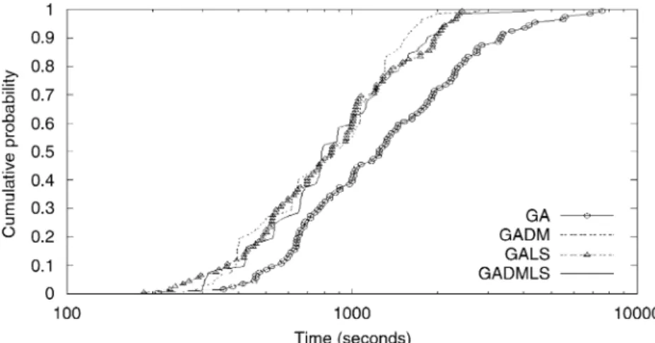
In another experiment, the objective was to verify the empirical probability distribution of reaching a given solution target value (i.e. find a solution with value as good as the target solution value) in function of time, for different algorithms. In this experiment we try to assess how fast these algorithms can generate good solutions. For this experiment, a bigger instance was created: d657_1000000_70. The solution values were chosen in a way that the slowest algorithm could terminate in a reasonable amount of time. Execution times of 100 independent runs were computed. The experiment design follows the proposal of[3]. Results of each algorithm were plotted (Fig.5) by associating theith smallest running time
rti with the probabilitypi¼ ði0:5Þ=100, which generates
points i¼ ðrti;piÞ, for i¼1;. . .;100. A simple analysis of
results can be done considering the alignment of curves: leftmost aligned curves indicate an algorithm with faster convergence, while rightmost aligned curves indicate slower algorithms. The results show that the simplest version (GA) takes considerably more time to achieve high cumulative probability values (40:5). Versions with DM
and/or local search perform much faster. There is a probability of 50% of GA to reach the target at 1,250 seconds, while for other algorithms it takes approximately 850 s, as shown inFig. 5.
To validate our experiments, we used the ILOG CPLEX 9.0 [16] to optimally solve the proposed instances. It successfully solved all problems generated from ulysses22 TSP-Library instance. Nevertheless, for bigger problems (48 and 70 nodes), the solver unexpectedly halted after some days of processing, when memory consumption was too high (greater than 10 Gigabytes). Optimal solution
values are shown in Table 3. Our heuristic methods, with DM and local search, always produced optimal solutions for three of four instances with known optimal solutions.
4. Conclusions and future works
In this work we presented three improved versions of an evolutionary algorithm. Versions which include local search and/or data mining (DM) were presented. Although applications of genetic algorithms (GAs) with local search
are abundant in the literature, the application of DM to improve the results of evolutionary algorithms is still scarce. The DM module proposed corresponds to an intensification strategy, since it tries to discover good features in the best solutions found so far and to apply them in the generation of new solutions. The addition of the DM module into the GA significantly improved this method and the hybrid version with local search (GADMLS), on average, produced the better results. Results could be improved if other interactions between modules and/or a more exhaustive set of experiments were conducted (perhaps, larger running times would benefit the more computationally expensive version—GADMLS). Nonetheless, our proposal looks very promising, specially considering problems in which it is difficult to devise efficient local search algorithms.
Since these hybrid versions consume considerable computational resources, an interesting future work is the development of parallel versions.
Table 2
Results for 10 independent executions for different problems (solution values multiplied by 103)
P. Id. GA GADM GALS GADMLS
Average Std. Dev. Average Std. Dev. Average Std. Dev. Average Std. Dev.
1 8.40 0.03 8.40 0.03 8.41 0.00 8.41 0.00
2 11.31 0.00 11.31 0.00 11.36 0.10 11.45 0.12
3 746.19 3.69 745.37 3.25 759.15 0.00 759.15 0.00
4 1,117.19 16.28 1,124.79 8.86 1,141.91 0.00 1,141.91 0.00
5 13.10 0.28 13.18 0.08 14.02 0.27 13.99 0.28
6 18.92 0.16 19.02 0.24 19.64 0.15 19.70 0.16
7 1,270.40 13.43 1,308.53 22.53 1,352.57 19.72 1,346.40 18.89
8 1,851.49 18.06 1,862.42 32.19 1,943.11 26.65 1,945.70 17.88
9 15.61 0.35 15.75 0.47 16.80 0.27 16.82 0.20
10 24.84 0.41 25.33 0.33 26.26 0.51 26.33 0.54
11 1,762.64 44.00 1,779.50 14.11 1,907.32 37.24 1,913.16 26.12
12 2,487.01 27.35 2,488.42 49.14 2,656.04 50.52 2,667.70 42.24
13 30.61 0.55 30.81 0.63 32.58 0.76 32.50 0.70
14 46.37 1.13 46.39 0.78 48.16 0.54 48.11 0.88
15 2,980.01 75.93 3,009.10 61.25 3,118.62 49.14 3,188.91 89.06
16 4,511.45 68.03 4,585.47 77.92 4,738.50 96.30 4,765.40 49.70
17 35.65 0.87 36.01 0.62 38.93 0.72 39.37 0.55
18 67.31 0.72 67.65 0.83 70.84 0.85 70.39 0.95
19 3,810.39 55.55 3,878.00 83.29 4,025.35 90.83 4,033.73 36.44
20 7,384.82 85.15 7,450.16 103.09 7,773.92 98.03 7,789.02 121.83
21 46.84 0.53 47.96 1.29 50.06 0.92 49.80 1.23
22 78.07 0.97 78.76 1.73 83.16 1.38 83.58 1.41
23 4,986.12 132.21 4,914.60 56.48 5,265.43 118.35 5,292.82 170.79
24 8,258.49 86.84 8,429.63 155.41 8,817.44 160.33 8,708.05 101.63
25 91.78 1.69 91.44 1.29 96.34 1.07 94.68 1.10
26 138.83 1.28 142.43 1.06 144.37 1.67 143.53 1.69
27 9,588.19 244.18 9,750.25 128.91 10,033.14 240.47 10,029.48 309.57
28 14,344.72 108.31 14,491.22 153.81 14,848.62 139.11 14,763.11 134.69
29 82.30 1.24 82.17 1.51 86.71 1.34 87.16 1.68
30 132.15 1.69 133.29 2.04 138.05 1.52 136.61 1.55
31 8,288.89 135.66 8,194.22 160.61 8,709.20 187.28 8,605.22 102.23
32 12,958.52 172.69 13,198.49 315.53 13,526.36 78.17 13,670.47 196.76
33 124.29 1.56 125.86 2.21 128.19 2.51 127.48 1.84
34 176.58 1.53 177.11 0.95 178.59 2.28 179.57 2.09
35 12,483.73 201.48 12,531.07 150.40 12,620.18 192.57 12,624.20 254.79
36 17,661.23 162.54 17,693.57 182.05 17,853.19 138.80 17,876.98 143.68
Table 3
Optimal solutions (solution values multiplied by 103)
Problem Optimal solution
ulysses22_1000_40 8.41
ulysses22_1000_70 11.56
ulysses22_1000000_40 759.15
Acknowledgments
The authors are grateful to CNPq and CAPES that partially funded this research. Also, authors would like to thank the referees, for their valuable comments and Professor Eduardo Uchoa (Universidade Federal Flumi-nense) and Olinto C. Bassi Araujo (DENSIS-FEE-UNI-CAMP), for their help with computational resources and software for this research.
References
[1] R. Agrawal, R. Srikant, Fast algorithms for mining association rules, in: Proceedings of 20th International Conference on Very Large Data Bases VLDB, Morgan Kaufmann, Loss Altos, CA, 1994, pp. 487–499. [2] R. Agrawal, R. Srikant, Mining sequential patterns, in: Proceedings
of 11th International Conference on Data Engineering, 1995, pp. 3–14.
[3] R.M. Aiex, M.G.C. Resende, C.C. Ribeiro, Probability distribution of solution time in GRASP: an experimental investigation, J. Heuristics 8 (2002) 343–373.
[4] E. Balas, The prize collecting traveling salesman problem, Networks 19 (1989) 621–636.
[5] J. Berger, M. Barkaoui, A new hybrid genetic algorithm for the capacitated vehicle routing problem, Oper. Res. Soc. 54 (2003) 1254–1262.
[6] J.L. Bresina, Heuristic-biased stochastic sampling, in: Proceedings of the Thirteenth National Conference on Artificial Intelligence, Port-land, 1996, pp. 271–278.
[7] T. Feo, M. Resende, Greedy randomized adaptive search procedures, J. Global Optim. 6 (1995) 109–133.
[8] P. Galinier, J. Hao, Hybrid evolutionary algorithms for graph coloring, J. Combin. Optim. 3 (4) (1999) 379–397.
[9] M.N. Garofalakis, R. Rastogi, K. Shim, Mining sequential patterns with regular expression constraints, IEEE Trans. Knowl. Data Eng 14 (3) (2002) 530–552.
[10] A. Ghosh, A. Freitas, Special issue on data mining and knowledge discovery with evolutionary algorithms, IEEE Trans. on Evol. Comput. 7 (6) (2003) 450.
[11] D.E. Goldberg, Genetic Algorithms in Search, Optimization and Machine Learning, Addison-Wesley, Menlo Park, 1989.
[12] B.L. Golden, L. Levy, R. Vohra, The orienteering problem, Naval Res. Logist. 24 (1987) 307–318.
[13] G. Gutin, A.P. Punnen (Eds.), Traveling Salesman Problem and Its Variations, Springer, Berlin, 2002.
[14] J. Han, K. Micheline, Data Mining: Concepts and Techniques, Morgan Kaufmann Publishers, Los Altos, CA, 2000.
[15] J.H. Holland, Adaptation in Natural and Artificial Systems, University of Michigan Press, Ann Arbor, 1975.
[16] ILOG S.A. ILOG CPLEX 9.0: User’s Manual, 2003.
[17] J.K. Lenstra, E.H.L. Aarts (Eds.), Local Search in Combinatorial Optimization, Wiley, New York, 1997.
[18] M. Matsumoto, T. Nishimura, Mersenne twister: A 623-dimension-ally equidistributed uniform pseudorandom number generator, ACM Trans Model. Comput. Simul. 8 (1) (1998) 3–30.
[19] D. Mester, O. Braysy, Active guided evolution strategies for large scale vehicle routing problems with time windows, Comput. Oper. Res. 32 (2005) 1593–1614.
[20] P. Moscato, On evolution, search, optimization algorithms and martial arts: towards memetic algorithms, Technical Report 826, California Institute of Technology, Pasadena, 1989.
[21] P. Moscato, C. Cotta, Handbook of Metaheuristics, A Gentle Introduction to Memetic Algorithms, Kluwer Academic Press, Boston, 2003, pp. 105–144.
[22] A.J. Orman, H.P. Willians, A survey of different integer program-ming formulations of the travelling salesman problem, Technical Report LSEOR 04.67, London School of Economics, London, 2004. [23] J. Pei, J. Han, Constrained frequent pattern mining: a pattern-growth
view, SIGKDD Explorations 4 (2002) 31–39.
[24] C. Prins, A simple and effective evolutionary algorithm for the vehicle routing problem, Comput. Oper. Res. 31 (2004) 1985–2002. [25] T. Ramesh, Traveling purchaser problem, Opsearch 18 (1981) 78–91. [26] C.R. Reeves, Modern heuristic techniques for combinatorial pro-blems, Genetic Algorithms, Wiley, New York, 1993, pp. 151–188. [27] G. Reineilt, Traveling Salesman Problemh
http://www.iwr.uni-heidel-berg. de/groups/comopt/software/TSPLIB95/i
[28] G. Reineilt, TSPLIB—A traveling salesman problem library, ORSA J. Comput. 3 (1991) 376–384.
[29] C.C. Ribeiro, M.G.C. Resende, Handbook of Metaheuristics, Greedy randomized adaptive search procedures, Kluwer Academic Publish-ers, MA, 2002, pp. 219–249.
Haroldo G. Santoshas received M.Sc. degree in Production Engineering from Universidade Fed-eral de Santa Maria in 2002. He is currently pursuing his D.Sc. degree in Computer Science at the Universidade Federal Fluminense, Brazil. His research interests include combinatorial optimi-zation: metaheuristics and integer programming and parallel computing.
Luiz S. Ochi is an Associate Professor of Computer Science at Universidade Federal Flu-minense, Brazil. He received his D.Sc. in Com-puter Science from the Universidade Federal do Rio de Janeiro, Brazil, in 1989. His research interest are in Combinatorial Optimization and Computational Intelligence.
Euler H. Marinhoreceived his M.Sc. degree in Computer Science from the Universidade Federal Fluminense, Brazil in 2005. His research interests include Operational Research, mainly Optimiza-tion Techniques applied in transport systems, and Metaheuristics.