J. Braz. Soc. Mech. Sci. & Eng. vol.33 número3

(1)

Heinsten F. L. dos Santos

hfleal@sc.usp.br Department of Mechanical Engineering São Carlos School of Engineering University of São Paulo 13566-590 São Carlos, SP, Brazil

Marcelo A. Trindade

trindade@sc.usp.br Department of Mechanical Engineering São Carlos School of Engineering University of São Paulo 13566-590 São Carlos, SP, Brazil

Structural Vibration Control Using

Extension and Shear Active-Passive

Piezoelectric Networks Including

Sensitivity to Electrical Uncertainties

Active-Passive Piezoelectric Networks (APPN) integrate active voltage sources with passive resistance-inductance shunt circuits to a piezoelectric patch. This technique allows to simultaneously passively dissipate vibratory energy through the shunt circuit and actively control the structural vibrations. This work presents an analysis of active-passive damping performance of beams with extension and shear APPN. A coupled finite element model with mechanical and electrical degrees of freedom is developed and used to design passive and active control parameters. Then, stochastic modeling and analyses of two cantilever beam configurations, with extension and shear APPN, are performed to evaluate the effect of uncertainties in circuit components on passive and active-passive vibration control. Results show that active-passive shunt circuits can be very interesting since they may combine an adequate passive control performance with an increase of active control authority when a control voltage is applied to the circuit. For the extension configuration, vibration amplitude reductions of up to 22 dB and 28 dB are obtained for passive and active-passive cases, respectively. Considering relative dispersions of 10% for the resistance and inductance values, the passive and active-passive amplitude reductions are found to be in the ranges 16-24 dB and 27-28 dB, respectively. For the shear configuration, increases in the active control authority of up to 29 dB due to a properly tuned resonant circuit are observed. When subjected to uncertainties in the resistance and inductance values, with 10% relative dispersions, the control authority increase is in the range of 6-29 dB. Keywords:piezoelectric materials, active-passive piezoelectric networks, vibration control, stochastic modeling, uncertainty analysis

Introduction

Due to their strong electromechanical coupling, piezoelectric materials have been widely used as sensors and actuators for structural vibration control. They can be used either as actuators connected to an appropriate control law to provide active vibration control or as sensors connected to shunt circuits to provide passive damping. In the last decade, research was redirected to combined active and passive vibration control techniques. One of these techniques, so-called Active-Passive Piezoelectric Networks (APPN), integrates an active voltage source with a passive resistance-inductance shunt circuit to a piezoelectric sensor/actuator (Tsai and Wang, 1999). In this case, the piezoelectric material serves two purposes. First, the vibration strain energy of the structure can be transferred to the shunt circuit, through the difference of electric potential induced in the piezoelectric material electrodes, and then passively dissipated in the electric components of the shunt circuit (Forward, 1979; Hagood and von Flotow, 1991, Viana and Steffen, 2006). On the other hand, the piezoelectric material may also serve as an actuator for which a control voltage can be applied to actively control the structural vibrations. This active mechanism combined to a velocity feedback, for instance, may then induce an additional active damping in the structure.

There are still some unresolved issues concerning this active-passive damping mechanism, such as for which conditions simultaneous active-passive damping outperforms separate active and passive mechanisms, that is, whether the control voltage should be part of the shunt circuit or not (Thornburgh and Chattopadhyay, 2003). It has been shown that combined active-passive vibration control allows better performance with smaller cost than separate active and passive control, provided the simultaneous action is

Paper received 5 August 2010. Paper accepted 5 February 2011. Technical Editor: Francisco Cunha

optimized (Tsai and Wang, 1999). On the other hand, like for purely passive shunted piezoelectric damping, most of the studies concerning APPN focus on the optimization of the electric circuit architecture and components. It is well-known, however, that the performance of both active and passive damping mechanisms is highly dependent on the effective electromechanical coupling provided by the piezoelectric actuators/sensors. Nevertheless, few studies focus on the optimization of this coupling for given structure and piezoelectric material. In particular, it has been shown that piezoelectric actuators using their thickness-shear mode can be more effective than surface-mounted extension piezoelectric actuators for both active (Trindade, Benjeddou and Ohayon, 1999; Raja, Prathap and Sinha, 2002; Baillargeon and Vel, 2005; Trindade and Benjeddou, 2006) and passive (Benjeddou and Ranger-Vieillard, 2004; Benjeddou, 2007; Trindade and Maio, 2008) vibration damping. One of the reasons for that is the thickness-shear electromechanical coupling coefficient k15 that is normally twice the value of the extension one, k31, which may lead to a higher effective electromechanical coupling coefficient (Trindade and Benjeddou, 2009). The thickness-shear mode, originally proposed by Sun and Zhang (1995), can be obtained using longitudinally-poled piezoelectric patches that couple through-thickness electric fields/displacements and shear strains/stresses. On the other hand, although it is well-known that the performance of shunt circuits is quite sensible to the tuning of circuit parameters, little has been published about the complexities in tuning the electric circuit parameters and the effect of the parametric variations on the overall performance of the system (Viana and Steffen, 2006; Andreaus and Porfiri, 2007).

(2)

circuit equations are also included in the variational formulation. Hence, conservation of charge and full electromechanical coupling are guaranteed. The formulation results in a coupled finite element model with mechanical (displacements) and electrical (electrodes charges) degrees of freedom. An analysis of the resulting coupled equations of motion is performed to identify the damping mechanisms provided by an active-passive piezoelectric network. Then, stochastic modeling and analysis of two cantilever beam configurations, with extension and shear piezoceramics, are performed to account for uncertainties in circuit components. This work includes an original modeling and analysis of APPN using shear response mode of piezoelectric materials and also an original sensitivity analysis of passive and active-passive shunted piezoelectric damping using a stochastic model.

Nomenclature

A = cross-sections or electrodes area

b = perturbation input distribution vector

C = damping matrix

c = output distribution vector

¯

cDk₁₁ = effective elastic stiffness constant of surface layer k

¯

cDc

33 = effective elastic stiffness constant of core layer D = vector of electric displacements dof

D3 = transverse electric displacement

E3 = transverse electric field

F = vector of generalized mechanical forces f = amplitude of perturbation input

Gc = control authority of pair patch and shunt circuit Gh = FRF for beams with active-passive shunt circuits Gp = FRF for beams with passive shunt circuits

g = vector of control gains H = electric enthalpy

¯

hk₃₁ = effective piezoelectric constant of surface layer k hc₁₅ = effective piezoelectric constant of core layer

h = thickness

I = second moment of cross-section area

K = stiffness matrix

¯

K = modified stiffness matrix

ke = effective stiffness coefficient of pair patch-circuit

kp = effective piezoelectric stiffness of vibration mode of interest L = length of the beam

Lc j = inductance of circuit j

M = mass matrix

mq = effective inertia coefficient of pair patch-circuit pX = probability density function of random variable X

qc = vector of electric charges generated at piezo-patches Rc j = resistance of circuit j

u = vector of nodal mechanical displacements u = axial displacement

T = kinetic energy

Vc j = voltage source applied to circuit j W = work done by dissipative forces w = transverse displacement y = mechanical response output

Greek Symbols

αn = modal displacement of vibration mode of interest ¯

βε₃₃k = effective dielectric constant of surface layer k

βε₁₁c = effective dielectric constant of core layer

βi = cross-section rotation angle

δ = virtual variation operator

δX = relative dispersion of random variable X

ε1 = normal strain

ε5 = shear strain

φn = vibration mode of interest

ω = resonance frequency

ρi = mass density of layer i

σ1 = normal stress

σ5 = shear stress

σX = standard deviation of random variable X

Subscripts

c = relative to electric shunt circuits

e = relative to dielectric contributions or electric circuit i = relative to layer i

j = relative to circuit j

L = relative to shunt circuit inductance m = relative to mechanical contributions me = relative to piezoelectric contributions n = relative to vibration mode n

p = relative to piezoelectric patch p q = relative to electric displacement dofs R = relative to shunt circuit resistance

Superscripts

c = relative to core layer or shear strain D = for constant electric displacement

ε = for constant strain f = relative to bending strain k = relative to surface layer k m = relative to membrane strain

OC = relative to open-circuited shunt circuit R = relative to resistive shunt circuit RL = relative to resonant shunt circuit SC = relative to short-circuited shunt circuit V = relative to voltage source only

Finite Element Model of a Piezoelectric Sandwich Beam

Consider a sandwich beam made of piezoelectric layers and modeled using a classical sandwich theory. Surface layers are made of transversely poled piezoelectric materials, whereas the core layer is made of longitudinally poled piezoelectric materials. Electrodes fully cover the top and bottom skins of all layers so that only through-thickness electric field and displacement are considered. For simplicity, all layers are assumed to be made of orthotropic piezoelectric materials, perfectly bonded and in plane stress state. Bernoulli-Euler theory is retained for the sandwich beam surface layers, while the core is assumed to behave as a Timoshenko beam. The length, width and thickness of the beam are denoted byL,band

(3)

Displacements and strains

The axial and transverse displacement fields of faces and core may be written in the following general form:

¯

ui(x,y,z) =ui(x) + (z−zi)βi(x), i=t,c,b,

¯

vi(x,y,z) =0,

¯

wi(x,y,z) =w(x),

(1)

whereuiis the mid-plane axial displacement of the layeri(i=tfor the top layer,i=cfor the core layer andi=bfor the bottom layer).βiis the cross-section rotation angle and from Bernoulli-Euler assumptions

βt=βb=−w′, wherew′states for∂w/∂x.zistates for the position of the layerimid-plane in the global transversalzdirection. Using the displacement continuity conditions between layers, the displacement fields may be written in terms of only three main variables,ut,uband w, so thatucandβcare written as

uc= ut+ub

2 +

hd 4w

′ _and _β

c= ut−ub

hc +hm

hc

w′, (2)

withhmandhd being the mean and difference of the surface layers thicknesses,htandhb:

hm= ht+hb

2 and hd=ht−hb. (3)

The usual strain-displacement relations for each layer yield the following axial and shear strains for the layeri:

ε1i= ∂_u_¯_i

∂_x =ε m

i + (z−zi)εif and ε5i= ∂_u_¯_i

∂_z + ∂_w_¯_i

∂_x =ε c i, (4)

while the remaining strainsε2i,ε3i,ε4iandε6ivanish. The membrane, bending and shear generalized strains,εm_i ,ε_if andεc_i, can be written as

εm_k =u′_k,ε_kf=−w′′,εc_k=0, for surface layers(k=t,b), (5)

εmc = u′_t+u′_b

2 +

hd 4w

′′_,_εf

c= u′_t−u′_b

hc +hm

hc w′′,

εcc= ut−ub

hc + hm hc +1 w′.

(6)

Alternatively, these expressions can be written in terms of the mean and relative axial displacements, instead of the axial displacements of the top and bottom layers, as done in previous works (Benjeddou, Trindade and Ohayon, 1999; Trindade, Benjeddou and Ohayon, 2001).

Piezoelectric constitutive equations

Linear orthotropic piezoelectric materials with material symmetry axes parallel to the beam ones are considered here. The constitutive equations for these materials can be obtained starting from the general expression for the electric enthalpy of a piezoelectric layer

H(ε,D) =1 2ε

t_cD_ε₋_εt_ht_D₊1 2D

t_βε_D_, ₍₇₎

such that

σ=∂_H_/∂_ε₌_cD_ε₋_ht_D_,

E=∂_H_/∂_D₌₋_h_ε₊_βε_D_, (8)

wherecD_{i j}, hl j and βεl (i,j=1, ...,6;l=1,2,3) denote the elastic (for constant electric displacement), piezoelectric and dielectric (for constant strain) constants of the piezoelectric material, respectively.

For both extension and shear mode piezoelectric layers, only transverse electric field and displacements are considered (D1=D2= 0) since the layers have electrodes on top and bottom skins. However, faces and core layers are treated separately, since they have different poling directions. An additional assumption of plane stress state (σ3=0) allows to write the following reduced constitutive equations for the faces and the core:

σ1k E3k

=

¯

cDk₁₁ −h¯k₃₁ −h¯k₃₁ β¯εk

33

ε1k D3k

, (9) and   

σ1c

σ5c E3c

  =   ¯

cDc₃₃ 0 0

0 cDc₅₅ −hc₁₅

0 −hc₁₅ βε₁₁c  

  

ε1c

ε5c D3c

 

, (10)

where,

¯

cDk₁₁ =cDk₁₁−c

Dk 13 2

cDk₃₃ ,

¯

hk₃₁=hk₃₁−hk₃₃c Dk 13

cDk₃₃,

¯

βε₃₃k=βε₃₃k+h k 33

2

cDk₃₃ , (11)

¯

cDc₃₃ =cDc₃₃₋c Dc 132

cDc₁₁ . (12)

Finite element discretization

Lagrange linear shape functions are assumed for the axial displacements,ut andub, and electric displacements in each layer, D3t, D3c andD3b. For the transverse deflectionw, Hermite cubic shape functions are assumed. These assumptions lead to a two node finite element with four mechanical dof and three electrical dof per node. The elementary mechanical degrees of freedom (dof) column vectorunis defined as

un= [u(t1) u

(1)

b w

(1) _w′(1) _u(2)

t u

(2)

b w

(2) _w′(2)_]t_.

(13)

The axial and transverse displacements of the face layers can be written in terms of the elementary dofs as

uk=Nxkun,w=Nzun,k=t,b, (14)

where

Nxt=

N1 0 0 0 N2 0 0 0

,

Nxb=

0 N1 0 0 0 N2 0 0

,

Nz=

0 0 N3 N4 0 0 N5 N6

,

(15)

(4)

N1=1−

x L,N2=

x

L,N3=1−

3x2 L2 +

2x3 L3,N4=x

1−x L

2

,

N5=

x2 L2

3−2x L

,N6=

x2 L

_x

L−1

.

(16)

The axial displacement of the core layerucand the cross-section rotationsβican then be written, usingβt=βb=−w′and (2), as

uc=Nxcun,βi=Nriun,i=t,c,b, (17)

where

Nxc=

Nxt+Nxb

2 +

hd 4N

′ z,Nrc=

Nxt−Nxb hc

+hm

hc

N′_z,

Nrt=N′xt,Nrb=N′xb.

(18)

According to expressions (5) and (6) for the generalized strains,

εm i ,ε

f

i, andεci, they can be written in terms of the elementary dofs as

εmi =Bmiun,εif=Bf iun,εcc=Bccun. (19)

The membrane, bending and shear strain operatorsBmi,Bf iand

Bccare defined as

Bmi=N′xi,Bf i=Nri′,Bcc=Nrc+N′z. (20)

The elementary electric dofs column vectorDnis defined as

Dn=

h

D₃(1_t) D(₃1_c) D(₃1_b) D(₃2_t) D(₃2_t) D(₃2_b) it

. (21)

Then, the electric displacement in the piezoelectric layers can be written in terms of the elementary dofs

D3i=NDiDn,i=t,c,b, (22)

where

NDt=

N1 0 0 N2 0 0

,

NDc=

0 N1 0 0 N2 0

,

NDb=

0 0 N1 0 0 N2

.

(23)

Variational formulation

The equation of motions can be written using the Hamilton’s principle extended to piezoelectric media

δΠ_b=

Z

t

"

∑

i

(δTi−δHi) +δWm

#

dt=0, (24)

whereδTi,δHiandδWmare the virtual variations of kinetic energyTi and electric enthalpyHiof layeriand the total virtual work done by mechanical forces on the structure.

The virtual variation of kinetic energy for layeriof the sandwich beam can be written using the displacements fields defined in (1) and supposing that all layers are symmetric with respect to their neutral lines,z=zi, such that integration over the cross-section areas leads to

Z

t

δTidt=−

Z

t

ZL

0

ρiAi(δuiu¨i+δww¨) +ρiIiδβiβ¨i

dxdt, (25)

whereρiis the mass density andAiandIi are the area and second moment of area of the cross-section of layeri, respectively, and the dot stands for time derivation.

Using the finite element discretization of generalized displacements (14) and (17),

Z

t

δTidt=−

Z

t

δutnMiu¨ndt, (26)

whereMiis mass matrix of the layeridefined as

Mi=

ZL

0

ρiAi(NtxiNxi+NzitNzi) +ρiIiNtriNri

dx. (27)

The virtual variation of the electric enthalpyHifor each layer will be composed of mechanicalδHmi, electromechanical (piezoelectric)

δHmei, and dielectricδHeicontributions. In what follows, these are detailed for the facesi=t,band corei=clayer.

For the core layer, both normal and shear strains contribute to the virtual variation of electric enthalpy, while for the faces only normal strains are relevant. Then, using (4) and supposing symmetric layers, the integration over the cross-section reducesδHmito

δHmk=

ZL

0

δεm_kc¯Dk11Akεmk+δε f kc¯

Dk 11Ikε_kf

dx,k=t,b,

δHmc=

ZL

0

δεmcc¯Dc33Acεmc+δε f

cc¯Dc33Icεcf+δεcckccDc55Acεcc

dx,

(28)

wherekcis a shear correction factor for the Timoshenko core layer. Also supposing symmetric layers and integrating in the cross-section, the piezoelectric contributions to the virtual variation of electric enthalpy can be written as

δHmek=−

ZL

0

δεm_kh¯k₃₁AkD3k+δD3kh¯k31Akεmk

dx,

δHmec=−

ZL

0

(δεc_chc₁₅AcD3c+δD3chc15Acεcc)dx.

(29)

Notice that the piezoelectric effect couples the transversal electric displacementD3iwith membrane and bending strainsεm_k andε_kf, for the faces, and with shear strainεc

c, for the core.

The dielectric contribution to the virtual variation of electric enthalpy can be written as

δHek=

ZL

0

δD3kβ¯ε33kAkD3kdx, δHec=

ZL

0

δD3cβε11cAcD3cdx.

(30)

(5)

form substituting the discretized generalized strains (19) and electric displacements (22) in equations (28), (29) and (30), such that

δHmi=δutnKmiun,δHmei=−δutnKmeiDn−δDtnKtmeiun,

δHei=δDtnKeiDn,

(31)

whereKmiare the elastic stiffness matrices of the layeriwritten as

Kmk=

ZL

0

Bt_mkc¯Dk₁₁AkBmk+Btf kc¯Dk11IkBf k

dx,

Kmc=

ZL

0

Bt_mcc¯Dc₃₃AcBmc+Btf cc¯33DcIcBf c+BtcckccDc55AcBcc

dx,

(32)

Kmeistates for the electromechanical (piezoelectric) stiffness matrices

Kmek=

ZL

0

Bt_mkh¯k31AkNDk

dx,

Kmec=

ZL

0 B t

cch15AcNDc

dx,

(33)

andKeiare the dielectric stiffness matrices

Kek=

ZL

0

Nt_Dkβ¯ε₃₃kAkNDk

dx,

Kec=

ZL

0

Nt_Dcβε₁₁cAcNDc

dx.

(34)

The virtual work done by external mechanical forces can be written in terms of a vector of generalized mechanical forcesFsuch that

δWm=δutnF. (35)

Replacing the discretized virtual work expressions in the Hamilton’s principle (24) and assembling for all finite elements in the structure, the global equations of motion can be expressed as

M 0 0 0 ¨ u ¨ D +

Km −Kme

−Kt_me Ke

u D = F 0 , (36)

where u and D are the global mechanical and electric dofs and the mass and stiffness matrices and mechanical force vector were assembled for all layers and all finite elements.

Connecting Piezoelectric Patches to Electrodes and Electric Circuits

To account for the electrodes fully covering the piezoelectric patches top and bottom skins, the electric displacements of selected nodes and layers are set to be equal. This dof assignment can be represented by the following expression:

D=LpDp,Dp=Dp1 Dp2 ··· Dpnt (37)

where Lp is a binary matrix and Dp is a vector of the electric displacement for one piezoelectric patch (constant throughout the

electrode surface). Substituting (37) into the variational form of (36), the equations of motion are reduced to

M 0 0 0 ¨ u ¨ Dp +

Km −K¯me

−_K¯t me K¯e

u Dp = F 0 , (38) where ¯

Kme=KmeLp,K¯e=LtpKeLp. (39)

In addition, it is supposed that each piezoelectric actuator/sensor can be connected to an electric circuit composed of an inductanceLc j, a resistanceRc j and a voltage sourceVc j in series, with j=1, ...,n wherenis the number of electric circuits. The equations of motion for the circuits can be written using the Hamilton’s principle also as

δΠc=

Z

t n

∑

j=1

(δTc j+δWr j+δWe j)dt=0 (40)

whereδTc j,δWr jandδWe jare, respectively, the virtual variation of the kinetic energy due to the inductancesLc j and the virtual work done by the resistancesRc j and voltage sourcesVc j connected in series for the j-th electric circuit. These are written as

Z

t

δTc jdt=−

Z

t

δqt_{c j}Lc jq¨c jdt,δWr j=−δqtc jRc jq˙c j,

δWe j=δqtc jVc j, j=1, . . . ,n.

(41)

To account for the connection between piezoelectric patches and electric circuits, it is supposed that electric charges entering a given electric circuit are equal to electric charges of a given piezoelectric patch. Since, due to equipotentiality condition in the electrodes, the electric displacement is constant throughout the electrode surface, the electric charges for a given piezoelectric patch is obtained by multiplying the electric displacement by the electrode area. Thus, a diagonal matrixApwith elements that are the electrodes areas of each piezoelectric patch is defined. Then, the vector of electric charges generated at the piezoelectric patches and, thus, entering thenelectric circuits can be written as

qc=ApDp (42)

Including the virtual works of (41) in the variational form of the equations of motion (38) leads to

δut Mu¨+Kmu−K¯meDp−F

+δDtp −K¯tmeu+K¯eDp

+δqtc(−Lcq¨c−Rcq˙c+Vc) =0. (43)

Accounting for the relation between circuits’ electric charges and patches’ electric displacements (42), the structure-patches-circuits coupled equations of motion can then be written as

M 0

0 Mq

¨ u ¨ Dp + C 0

0 Cq

˙ u ˙ Dp +

Km −K¯me

−_K¯t me K¯e

u Dp = F Fq , (44)

(6)

Passive and Active Vibration Control Design

From (44), it is possible to observe that the shunt circuit can affect the structural response either passively through coupling of the dynamics of circuit and structure, via the piezoelectric patches, or actively through the application of an electric voltage in the circuit which excites the structure, also via the piezoelectric patches. These effects can be better observed in a frequency response function (FRF) of the structure when subjected to a mechanical or electrical excitation.

For a purely mechanical excitation, such that V_c₌_{0 and} _F₌ bf e˜ jωt_{, the amplitude of a displacement output}_y₌_cu_{can be written} such that ˜y=Gp(ω)f˜, where the FRFGp(ω)is

Gp(ω) =c

−ω2M+jωC+Km

−_K¯_me₍₋_ω2_M

q+jωCq+K¯e)−1K¯tme − 1

b, (45)

from which it is possible to notice that the resistance and inductance have the effect of changing the dynamic stiffness of the structure. Two particular cases of interest can be derived: i) open-circuit whenCq→

∞and ii) short-circuit whenMq=Cq=0, in which cases

GOCp (ω) =c

n

−ω2M+jωC+Km

o₋1 b,

GSCp (ω) =c

n

−ω2M+jωC+Km−K¯meK¯−e1K¯tme

o₋1 b.

(46)

As expected, no structural modification is observed in the open-circuit case while, for the short-open-circuit case, the stiffness of the piezoelectric patches is reduced.

For a purely electric excitation using a single pair patch-circuit, such thatF=0 andVc=V˜cejωt, the FRF between the outputyand the applied voltageVcis such that ˜y=Gc(ω)V˜c, where

Gc(ω) =c

−ω2M+jωC+Km

−_K¯_me₍₋_ω2

Mq+jωCq+K¯e)−1K¯tme − 1

×_K¯_me₍₋_ω2_M

q+jωCq+K¯e)−1Atp (47)

In this case, the resistance and inductance of the electric circuit have two effects. The first is a modification on the dynamic stiffness of the structure as in the previous case. The second is a modification of amplitude of the equivalent force input induced in the structure by the applied voltage, which for a properly adjusted circuit can lead to a desirable amplification of the control authority of the pair patch-circuit. The particular case of a simple voltage actuator can be derived by makingMq=Cq=0, for which

GV_c(ω) =c

n

−ω2M+jωC+Km−K¯meK¯−e1K¯tme

o₋1 ¯

KmeK¯−e1Atp

(48)

Passive vibration control using electromechanical vibration absorbers

Starting from the equations of motion (44) for the case of a single passive electric shunt circuit (RL) connected to a piezoelectric patch embedded in the structure, it is desired to apply the theory

of dynamic vibration absorbers for a particular vibration mode of interest. Therefore, the structural response is approximated by the contribution of a single vibration mode of interest such that

u(t) =φnαn(t), (49)

where φn and αn are the vibration mode of interest and its corresponding modal displacement. Thus, neglecting the structural damping, the equations of motion for the resulting two degree of freedom system can be written as

¨

αn+ω2nαn−kpDp=bnf,

mqD¨p+cqD˙p+keDp−kpαn=0,

(50)

whereφt

nMφn=1,φtnKmφn=ω2n,kp=φtnK¯meandbn=φtnb. Assuming a mechanical excitation through inputf, the structural response measured by a displacement outputy=cnαn, wherecn=

cφn, can be written such that its amplitude is ˜y=Gp(ω)f˜, where the amplitude of the FRFGp(ω)is

|Gp(ω)|=cnbn

h

(−ω2mq+ke)2+ (ωcq)2

i1/2

× n

[ω4mq−ω2(ke+mqωn2) +keωn2−kp2]2

+ [(−ω2+ωn2)ωcq]2

o₋1/2

. (51)

For limited values ofcq,|Gp(ω)|has an anti-resonance at a frequency equal to the resonance frequency of the electrical circuit, defined asωe= (ke/mq)1/2, which can be designed to match the structural resonance of interestωn. This leads to an expression formq, and thus for the inductanceLc, in terms ofωn, such that

Lc= ke

ω2 nA2p

, (52)

whereApis the surface area of the electrode covering the piezoelectric patch connected to the circuit. From the theory of dynamic vibration absorbers, it is known that the anti-resonance is accompanied by two resonances which may have their amplitudes controlled by the electric circuit dampingcq. One strategy to design the damping parameter is to minimize the difference between the resonances and anti-resonance amplitudes. This can be done by first using limcq→0|Gp(ω)|

2₌

limcq→∞|Gp(ω)|

2_{to find the frequencies for which the amplitude is}

independent of damping parameter which are

ω2₁_,₂= 1 2

h

ω2e+ω2n±

q

(ω2

e−ω2n)2+2ω2e(k2p/ke)

i

. (53)

Equalizing the vibration amplitudes at one of these invariant frequenciesω1and at the anti-resonance frequencyωn leads to an expression for the resistanceRcin terms of the equivalent coupling stiffnesskp, electrical stiffnesske, surface area of the electrodeAp and structural resonance frequency of interestωn,

Rc= kp

√

2ke

ω2 nA2p

(7)

Active vibration control using piezoelectric actuators and state feedback

A state feedback LQR (Linear Quadratic Regulator) optimal control is considered. For that, it is necessary to rewrite the equations of motion (44) in state space form, such that a vector of state variables zis defined, containing the modal displacements and velocities of a series of vibration modes of interest and the electric displacements of the piezoelectric patches and their time-derivatives. This leads to

˙

z=Azˆ +BVˆ c+Bˆff,y=Cˆyz, (55)

where

z=

    α

Dp ˙

α

˙ Dp

   ,Aˆ =

   

0 0 I 0

0 0 0 I

−Ω2 Kp −Λ 0

M−q1Ktp −Ωe2 0 −Λe

   ,

ˆ B=

   

0 0 0 M−1

q Atp

   ,Bˆf =

   

0 0 bφ

0

   ,Cˆy=

cφ 0 0 0

.

(56)

The modal displacements are such thatu=Φα and, for mass normalized vibration modes,Ω2₌_Φt_K

mΦand Λ=ΦtCΦ. Ω is a diagonal matrix which elements are the undamped natural frequencies of the structure with piezoelectric patches in open-circuit.

Ωe2=M−q1K¯eandΛe=M−q1Cq are both diagonal matrices which elements stand, respectively, for the squared natural frequencies of the electric circuits and the ratio between the resistances and inductances (M−_q1Cq=L−c1Rc). The electromechanical coupling stiffness matrix projected in the undamped modal basis is defined asKp=ΦtK¯me. Inputband outputcdistribution vectors are also defined, with modal projectionsbφ=Φtbandcφ=cΦ, andfis a vector of the amplitudes of each mechanical force applied to the structure.

A linear state feedback for the applied voltagesVcis assumed such thatVc=−gz=−gdmα−gdeDp−gvmα˙−gveD˙p, wheregis a vector of control gains for each state variable. Therefore, the state space equation (55) becomes

˙

z= (Aˆ−_Bgˆ ₎_z₊_Bˆ_f_f_,_y₌_Cˆ_y_z_. ₍₅₇₎

For a single-input mechanical excitation f, the closed-loop or controlled amplitude of a single displacement outputycan be written such that ˜y=Gh(ω)f˜, where the FRFGh(ω)is

Gh(ω) =Cˆy(jωI−Aˆ+Bgˆ )−1Bˆf, (58)

which can also be derived from the second order equations of motion projected into the undamped modal basis leading to

Gh(ω) =cφ

−ω2I+jω(Λ+KpD−cc1Atpgvm)

+ [Ω2+KpD−cc1(Atpgdm−Ktp)] − 1

bφ, (59)

where the closed-loop dynamic stiffness of the electric circuitDccis

Dcc=−ω2Mq+jω(Cq+Atpgve) + (K¯e+Atpgde). (60)

In this work, the control gaingis calculated using the standard optimal LQR control theory applied to a single-input/single-output case, that is, with only one active-passive patch-circuit pair for the control to minimize the vibration amplitude at one specific location of the structure, such that the following objective function is minimized:

J=1 2

Z∞

0

˙

y2+rV_c2dt, (61)

where ˙yis the velocity at one location of interest andVcis the control voltage applied to the active-passive shunt circuit. The weighting factorr is automatically adjusted to guarantee a maximum control voltage of 200V in all cases following an iterative routine proposed in (Trindade, Benjeddou and Ohayon, 1999).

Results and Discussion

In this section, the FRFs of two cantilever beam configurations, with extension and shear piezoceramics as shown in Figure 1, are analyzed in order to evaluate the APPN performance in terms of passive damping, control authority and active-passive damping. The extension and shear piezoceramics are made of PZT-5H material whose properties are: ¯cD

11=97.767 GPa, ¯cD33=119.71 GPa, cD55= 42.217 GPa,ρ=7500 kg m−3, piezoelectric coupling constants ¯h31=

−1.3520 109 N C−1 and h15=1.1288 109 N C−1, and dielectric constants ¯βε₃₃=57.830 106 m F−1 andβε₁₁=66.267 106 m F−1. For the Aluminium beam, material properties are: Young’s modulus 70.3 GPa and density 2710 kg m−3 and, for the foam, Young’s modulus 35.3 MPa, shear modulus 12.7 MPa and density 32 kg m−3. A viscous damping of 0.5% and a shear correction factorkc=0.83 were considered.

25

220

3.0 0.5

Piezoceramic _Aluminum

10

L R

source Voltage Shunt circuit

Output

External input Control input

(a)

25

220

3.0 0.5

Piezoceramic Aluminum

Aluminum 3.0 Foam

10

L R

source Voltage Shunt circuit Control input

Output

External input

(b)

Figure 1. Representation of cantilever beams with piezoceramic patches: (a) in extension and (b) in shear.

First, the beam with extension piezoelectric patch is analyzed. The resistance and inductance were tuned to the first resonance frequency, using the methodology presented in the previous section. Notice, however, that the values obtained using (52) and (54),Rc= 34117ΩandLc=406H, are just a first approximation to the optimal values and had to be fine-tuned manually to Rc =31541 Ω and Lc=390H. The purely passive action is obtained by eliminating the voltage source and the purely active action is obtained by making

Rc=Lc=0. For the general case, the inductance and resistance not only modify the dynamic stiffness of the structure, leading to damping and/or absorption, but also affects the active control authority of the actuator.

(8)

40 50 60 70 80 90100 200 300 400 ï60

ï50 ï40 ï30 ï20 ï10 0 10 20 30

Mobility (m/s/N, dB)

Frequency (Hz) OC

SC R RL

Figure 2. FRF of the beam with extension piezoceramic patch connected to a passive shunt circuit:GOC

p (dotted),GSCp (dashed),GRp(dash-dot) andGRLp

(solid).

40 45 50 55 60 65 70

−10 −5 0 5 10 15 20 25 30

Frequency (Hz)

OC

SC

R

RL

Figure 3. FRF, zoomed at the first resonance, of the beam with extension piezoceramic patch connected to a passive shunt circuit:GOC

p (dotted),GSCp

(dashed),GR

p(dash-dot) andGRLp (solid).

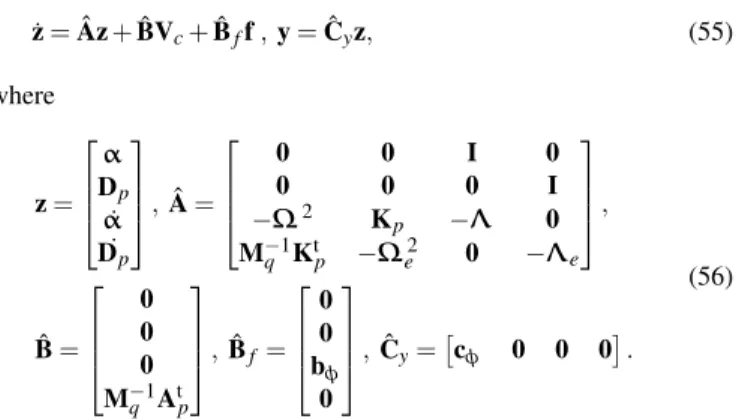
velocity when the beam is subject to a transverse force at the same point (Figure 2). The reference is considered to be unitary. It is possible to observe that both shunt circuits affect significantly only the first resonance, as expected. Figure 3 presents the same response, zoomed at the first resonance, from which one can conclude that both shunt circuits may yield a vibration amplitude reduction but the resonant circuit leads to a much better performance (approximately 22 dB vibration amplitude reduction). The resistive circuit leads to a variation in the resonance frequency, between short-circuit and open-circuit ones, and also induces an equivalent damping factor. For the resonant circuit, tuning of its resistance allows to reduce amplitude at the structure’s resonance frequency (i.e. the anti-resonance of the coupled system) at the cost of increasing the amplitude at the two resonance frequencies of the coupled system. Figure 4 shows the effect of increasing and decreasing the resistance of the optimal resonant circuit by 20%.

Figure 5 shows the active control authority of the piezoelectric material, acting as an actuator through the shunt circuit, measured as the beam tip velocity response when subject to a voltage applied to the circuit. As expected, the resistive shunt circuit diminishes the active control authority for all frequencies, since part of the input electric

40 45 50 55 60 65 70

−10 −5 0 5 10 15 20 25 30

Frequency (Hz)

OC

RL−

RL+

RL

Figure 4. FRF of the beam with extension piezoceramic patch connected to a resonant circuit subject to variations in the resistance value: open-circuit GOC

p (dotted), optimal RLGRLp (solid), RL with 20% reduction on resistance

valueGRL−

p (dashed) and RL with 20% increase on resistance valueGRL+p

(dash-dot).

40 50 60 70 80 90100 200 300 400

ï120

ï110

ï100

ï90

ï80

ï70

ï60

ï50

ï40

ï30

Mobility (m/s/V, dB)

Frequency (Hz) V

RV

RLVï

RLV+

RLV

Figure 5. Control authority of the extension piezoceramic patch: without shunt GV

c (dotted), resistive shunt GRc (fine dot), RL shunt with 20%

reduction on resistance valueGRL−

c (dashed), RL shunt with 20% increase

on resistance valueGRL+

c (dash-dot) and optimal RL shuntGRLc (solid).

40 45 50 55 60 65 70

−10 −5 0 5 10 15 20 25 30

Frequency (Hz)

OC

R

RV

RL

RLV

Figure 6. FRF of the beam with extension piezoceramic patch connected to passive and active-passive shunt circuits: open-circuitGOC

p (dotted),

passive R shuntGR

p(fine dot), active-passive R shuntGRh(dashed), passive

RL shuntGRL

(9)

80 100 200 300 400 500 600 700

ï70

ï60

ï50

ï40

ï30

ï20

ï10 0 10 20

Frequency (Hz) OC

SC

R

RL

Figure 7. FRF of the beam with shear piezoceramic patch connected to a passive shunt circuit: GOC

p (dotted),GSCp (dashed), GRp(dash-dot) andGRLp

(solid).

1020 103 104 105 106 107 108

2 4 6 8 10 12 14 16 18 20

Frequency (Hz)

OC

SC

R

RL

Figure 8. FRF, zoomed at the first resonance, of the beam with shear piezoceramic patch connected to a passive shunt circuit:GOC

p (dotted),GSCp

(dashed),GR

p(dash-dot) andGRLp (solid).

energy is being dissipated through the resistance. On the other hand, the resonant shunt circuit allows an increase of the active control authority around the first resonance at the cost of reducing it for the remaining frequency range.

Then, the LQR state feedback control strategy voltage presented previously was considered to evaluate the control voltage to be applied to the circuit and actively reduce the vibration amplitude of the beam. Figure 6 shows the beam tip mobility, zoomed at the first resonance, for uncontrolled beam (open-circuit, Rc→

∞), passive controlled beam with resistive (Rc =144 kΩ, Lc= 0, Vc=0) and resonant (Rc=31541 Ω, Lc=390 H, Vc=0) shunt circuits, and active-passive controlled beam with resistive (Rc= 144kΩ, Lc=0, Vc<200V) and resonant (Rc=31541Ω, Lc= 390 H, Vc <200 V) shunt circuits. The active-passive control yields better performance than its passive counterpart with amplitude reductions of approximately 14 dB (resistive) and 28 dB (resonant). Therefore, despite the small reduction on active control authority at the resonance frequency, active-passive control always outperforms the corresponding passive one.

Then, a similar analysis was performed for the sandwich beam with embedded shear piezoelectric patch. In this case, the resistance

1020 103 104 105 106 107 108

2 4 6 8 10 12 14 16 18 20

Frequency (Hz)

OC

RL−

RL+

RL

Figure 9. FRF of the beam with shear piezoceramic patch connected to a resonant circuit subject to variations in the resistance value: open-circuit GOC

p (dotted), optimal RLGRLp (solid), RL with 20% reduction on resistance

valueGRL−p (dashed) and RL with 20% increase on resistance valueGRL+p

(dash-dot).

80 100 200 300 400 500 600 700

ï120

ï110

ï100

ï90

ï80

ï70

ï60

ï50

ï40

ï30

ï20

Frequency (Hz) V

RV

RLVï

RLV+

RLV

Figure 10. Control authority of the shear piezoceramic patch: without shunt GV

c (dotted), resistive shuntGRc (fine dot), RL shunt with 20% reduction on

resistance valueGRL−

c (dashed), RL shunt with 20% increase on resistance

valueGRL+

c (dash-dot) and optimal RL shuntGRLc (solid).

1020 103 104 105 106 107 108

2 4 6 8 10 12 14 16 18 20

Frequency (Hz)

OC

R

RV

RL

RLV

Figure 11. FRF of the beam with shear piezoceramic patch connected to passive and active-passive shunt circuits: open-circuitGOC

p (dotted),

passive R shuntGR

p(fine dot), active-passive R shuntGRh(dashed), passive

RL shuntGRL

(10)

and inductance values obtained from (52) and (54) areRc=835.9Ω andLc=121.7H and were fine-tuned manually toRc=835.8Ω andLc=121.5H. The purely passive performance of resistive and resonant shunt circuits are presented in Figures 7 and 8. It is possible to observe that the vibration reduction performance is much smaller than in the previous case for both shunt circuits. This is due to the fact the sandwich design considered does not induce significant shear strains in the piezoelectric patch when the beam vibrates on the first mode. For the resonant circuit, the amplitude at structure’s first resonance can be further reduced by decreasing the resistance of the circuit as can be seen in Figure 9, which shows the effect of increasing and decreasing the resistance of the optimal resonant circuit by 20%. Figure 10 shows the active control authority of the shear piezoelectric patch, acting as an actuator through the shunt circuit, measured as the beam tip velocity response when subject to a voltage applied to the circuit. Here, the resistive shunt circuit also leads to a reduction on the active control authority for all frequencies. On the other hand, the resonant shunt circuit yields a very large increase on the active control authority around the first resonance. This fact indicates that, although the passive performance of the shear configuration is not very good, it might be an adequate choice for active or active-passive control since its control authority can be significantly enhanced by the circuit tuning. Indeed, as shown in Figure 11, when applying a similar LQR control strategy to the sandwich beam with shear actuator, the vibration amplitude is greatly reduced as compared to the corresponding passive case. As for the previous case, Figure 11 compares the frequency response of the beam when uncontrolled (open-circuit,Rc→∞), passive controlled with resistive (Rc=593kΩ, Lc=0,Vc=0) and resonant (Rc= 835.8Ω, Lc=121.5H,Vc=0) shunt circuits, and active-passive controlled with resistive (Rc=593 kΩ, Lc=0, Vc<200V) and resonant (Rc=835.8Ω,Lc=121.5H,Vc<200V) shunt circuits. The shear active-passive resonant control leads to an amplitude reduction of approximately 10 dB.

Stochastic Modeling for Uncertainties Analysis

This section presents an approach for analyzing random uncertainties for the resistanceRand inductanceLelements of the electric shunt circuits. An appropriate probabilistic model for each random variable,RbandbL, is constructed accounting for the available information only, which is the following: (1) the support of the probability density function is]0,+∞[; (2) the mean values are such thatE[R] =Rand E[L] =L; and (3) zero is a repulsive value for the positive-valued random variables which is accounted for by the condition E[ln(R)] =cR with |cR|<+∞ and E[ln(L)] =cL with

|cL|<+∞. Therefore, the Maximum Entropy Principle yields the following Gamma probability density functions forRandL(Soize, 2001; Cataldo et al., 2009; Ritto et al., 2010)

pR(R) =I]0,+∞[(R)

1

R

1

δ2 R

δ−2

R ₁

Γ(δ_R−2)

R R

δ−2 R−1

exp

− R

δ2 RR

(62)

and

pL(L) =I]0,+∞[(L)

1

L

1

δ2 L

δ−2

L ₁

Γ(δ_L−2)

L L

δ−2 L −1

exp

− L

δ2 LL

(63)

in whichδR=σR/RandδL=σL/Lare the relative dispersions of

b

RandbLandσR andσLare their standard deviations. The Gamma function is defined asΓ(α) =R₀∞tα−1e−tdt. These probability density functions are shown in Figure 12 together with the histograms of random sets forRandLgenerated with MATLAB functiongamrnd, considering 10000 realizations. The vectors of random realizations for Rb and bL where then combined into pairs of RL parameters, which were then applied to the evaluation of realizations of the FRF

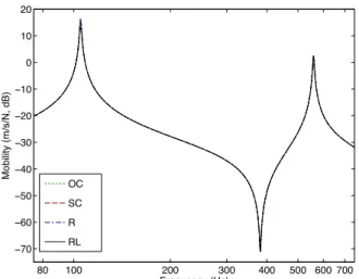
Gp(θj,ω), Gc(θj,ω)andGh(θj,ω)using equations (45), (47) and (58), respectively. To improve the analysis of the sensitiveness of the responses to the circuit parameters, three values were considered for the relative dispersions δR and δL: 5%, 10% and 20%. The mean-square convergence analysis with respect to the independent realizations of random variableGbp(ω), denoted byGp(θj,ω)was carried out considering the function

conv(ns) = 1

ns ns

∑

j=1

Z

kGp(θj,ω)−GNp(ω)k2dω, (64)

where ns is the number of simulations, or the number of RL pairs considered, and GNp(ω) is the response calculated using the corresponding mean model. Figure 13 shows the mean-square convergence analysis for extension and shear configurations consideringδR=δL=0.10. It is possible to observe that for both cases 3000 simulations are enough to assure convergence. Despite that, the statistical analyses presented in the following sections consider all 10000 simulations performed.

0.6 0.8 1 1.2 1.4

0 2 4

R/Rop

Probability density

0.6 0.8 1 1.2 1.4

0 2 4

L/Lop

Probability density

Figure 12. Probability density function for resistance (R/Rop) and inductance (L/Lop) values.

0 2000 4000 6000 8000 10000 0.4

0.6 0.8 1 1.2 1.4

Number of simulations

Normalized convergence

Figure 13. Mean square convergence of Monte Carlo simulation.

(11)

Rop

pR(R)

Gamma p.d.f. generator

Lop

pL(L)

Gamma p.d.f. generator

Computation of FRF

Convergence analysis

GN(ω)

G(ω), Gsup(ω), Ginf(ω)

Evaluation of mean and confidence interval of G(ω)

L(θj)

R(θj)

G(θj,ω)

y

n

Figure 14. Schematic procedure for the computation of FRFs mean and confidence intervals.

40 45 50 55 60 65 70

−5 0 5 10 15 20 25 30

Frequency (Hz)

Figure 15. FRF of the beam with extension piezoceramic patch connected to a passive shunt circuit:GOC

p (dash-dot),GNp(solid),Gp(dashed) andGCIp

(filled) forδR=δL=0.10.

30 40 50 60 70 80 90 100

−90 −80 −70 −60 −50 −40 −30

Frequency (Hz)

Figure 16. Control authority of the extension piezoceramic patch with and without shunt circuit:GV

c (dash-dot),GNc (solid),Gc(dashed) andGCIc (filled)

forδR=δL=0.10.

Figure 15 shows the FRFs for the extension configuration with OC (GOCp ) and RL shunted (GNp) piezoceramics, where, for last case, the nominal values ofR=31541Ωand L=390 H were used. It also shows the mean value (Gp) and 95% confidence intervals (GCIp ) of random variableGbp(ω)forδR=δL=0.10. Notice that the RL shunt circuit does not affect the FRF but near the first resonance (for which the shunt circuit was designed). In the FRF zoomed near the first resonance (Figure 15), one may notice that the nominal model

40 45 50 55 60 65 70

−5 0 5 10 15 20 25 30

Frequency (Hz)

Figure 17. FRF of the beam with extension piezoceramic patch connected to an active-passive shunt circuit:GOC

h (dash-dot),GNh (solid),Gh(dashed)

andGCI

h (filled) forδR=δL=0.10.

1038 103.5 104 104.5 105 105.5 106 106.5 107

9 10 11 12 13 14 15 16 17 18

Frequency (Hz)

Figure 18. FRF of the beam with shear piezoceramic patch connected to a passive shunt circuit:GOC

p (dash-dot),GNp(solid),Gp(dashed) andGCIp (filled)

forδR=δL=0.10.

90 95 100 105 110 115 120

−100 −90 −80 −70 −60 −50 −40 −30 −20

Frequency (Hz)

Figure 19. Control authority of the shear piezoceramic patch with and without shunt circuit:GV

forδR=δL=0.10.

(12)

1000 102 104 106 108 110 2

4 6 8 10 12 14 16 18 20

Frequency (Hz)

Figure 20. FRF of the beam with shear piezoceramic patch connected to an active-passive shunt circuit:GOC

h (dash-dot),GNh(solid),Gh(dashed) andGCIh

(filled) forδR=δL=0.10.

40 45 50 55 60 65 70

−5 0 5 10 15 20 25 30

Frequency (Hz) _(a)

40 45 50 55 60 65 70

−5 0 5 10 15 20 25 30

Frequency (Hz) _(b)

Figure 21. FRF of the beam with extension piezoceramic patch connected to a passive shunt circuit:GOC

p (dash-dot),GNp(solid),Gp(dashed) andGCIp

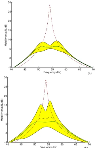
(filled) for: (a)δR=δL=0.05and (b)δR=δL=0.20.

found to be in the range 16-24 dB. It can be also noticed that the difference between the mean and nominal FRFs is almost negligible.

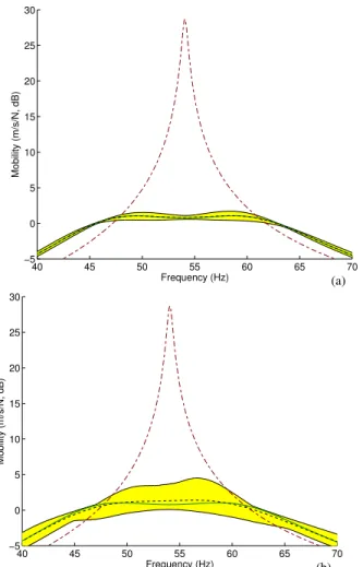
Then, an analysis of the control authority FRFs for the extension configuration with purely active (GVc) and RL shunted (GNc) was performed, including its mean (Gc) and 95% confidence intervals (GCIc ) forδR=δL=0.10. Figure 16 shows that despite the circuit

30 40 50 60 70 80 90 100

−90 −80 −70 −60 −50 −40 −30

Frequency (Hz) _(a)

30 40 50 60 70 80 90 100

−90 −80 −70 −60 −50 −40 −30

Frequency (Hz) _(b) Figure 22. Control authority of the extension piezoceramic patch with and without shunt circuit:GV

for: (a)δR=δL=0.05and (b)δR=δL=0.20.

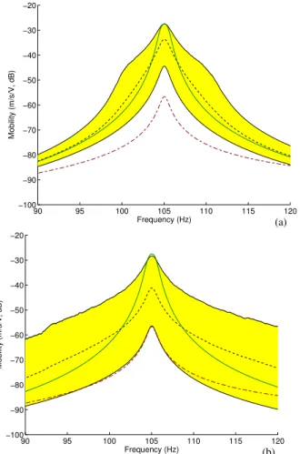
components uncertainties, the control authority is indeed increased near the first resonance at the cost of being significantly reduced for higher frequencies. The active-passive vibration control performance can be observed in Figure 17, which shows the FRFs for the uncontrolled (GOC_p ) and controlled structure (GN_h), including its mean (G_h) and confidence intervals (GCI_h ) forδR=δL=0.10. Comparison with Figure 15 shows that the LQR control combined with the resonant shunt circuit allows to reduce further the vibration amplitude. Indeed, the nominal model indicates a reduction of 27.5 dB, while the confidence intervals indicate a reduction between 27 dB and 28 dB. It is also worthwhile to notice that the active control also shrinks the confidence intervals, compared to the passive case.

Similar analyses were done for the shear configuration. Hence, Figure 18 shows the FRFs with OC (GOCp ) and RL shunted (GNp) piezoceramics. For the present shear case, the nominal values of

(13)

40 45 50 55 60 65 70 −5

0 5 10 15 20 25 30

Frequency (Hz) _(a)

40 45 50 55 60 65 70

−5 0 5 10 15 20 25 30

Frequency (Hz) _(b)

Figure 23. FRF of the beam with extension piezoceramic patch connected to an active-passive shunt circuit:GOC

h (dash-dot),GNh (solid),Gh(dashed)

andGCI

h (filled) for: (a)δR=δL=0.05and (b)δR=δL=0.20.

to a significant control authority amplification near the first resonance and, differently from the extension configuration, it occurs also at the resonance (Figure 19). This amplification leads to an increase of 29 dB at the resonance, according to the nominal model, and in the range{6-29}dB, according to the 95% confidence intervals. From Figure 20, the vibration amplitude reduction induced by the active-passive control is 10 dB, according to the nominal model, and between 3 dB and 11 dB, according to the 95% confidence intervals.

It is also worthwhile to analyse the effect of the relative dispersions of resistance and inductance values on the confidence intervals of the responses of passive and active-passive controlled structures and the control authority of the shunted piezoelectric actuators. Therefore, two additional values for relative dispersions

δR and δL were considered: 0.05 and 0.20. It is expected that higher relative dispersions would lead to wider confidence intervals and vice-versa. Figures 21, 22 and 23 show, respectively, the frequency responsesGp,GcandGhof the structure with the extension piezoceramics for the two additional relative dispersions. It can be observed in Figure 21, as expected, that the confidence interval is widened (shrunk) compared to the previous case (Figure 15) for larger (smaller) relative dispersions. The range of vibration amplitude reduction (considering the difference between peak responses) becomes 19-24 dB, for 5% relative dispersion, and 11-25 dB, for 20% relative dispersion. The same behaviour was observed for the control authority (Figure 22) and active-passive case (Figure 23). The range

1038 103.5 104 104.5 105 105.5 106 106.5 107

9 10 11 12 13 14 15 16 17 18

Frequency (Hz) _(a)

1038 103.5 104 104.5 105 105.5 106 106.5 107

9 10 11 12 13 14 15 16 17 18

Frequency (Hz) _(b)

Figure 24. FRF of the beam with shear piezoceramic patch connected to a passive shunt circuit:GOC

p (dash-dot),GNp(solid),Gp(dashed) andGCIp (filled)

of vibration amplitude reduction when using the active-passive shunt circuit remains 27-28 dB, for 5% relative dispersion, and is widened to 24-29 dB, for 20% relative dispersion.

Similar behaviour was also observed in an analysis performed for the shear actuated sandwich beam. The range of vibration amplitude reduction for the beam with shear piezoceramic patch connected to a passive resonant shunt circuit was 0-2.7 dB and 0-3.6 dB for 5% and 20% relative dispersions, respectively (Figure 24). In terms of control authority, as shown in Figure 25, increasing the resistance and inductance relative dispersions yields decreasing lower limit for the confidence intervals, 16 dB and 0 dB for 5% and 20% relative dispersions, respectively, while the upper limit remains unchanged (29 dB). The confidence intervals for the active-passive performance, in terms of vibration amplitude reduction, of the shear actuated piezoceramics are also widened when increasing the corresponding resistance and inductance relative dispersions and vice-versa. The range of vibration amplitude reduction for the active-passive shunted shear piezoceramics is 5-11 dB, for 5% relative dispersion, and 2-11 dB, for 20% relative dispersion.

Concluding Remarks

(14)

90 95 100 105 110 115 120 −100

−90 −80 −70 −60 −50 −40 −30 −20

Frequency (Hz) _(a)

90 95 100 105 110 115 120

−100 −90 −80 −70 −60 −50 −40 −30 −20

Frequency (Hz) _(b)

Figure 25. Control authority of the shear piezoceramic patch with and without shunt circuit:GV

model with mechanical and electrical degrees of freedom was developed and used to design passive and active control parameters. Then, a stochastic modeling and analysis of two cantilever beam configurations, with extension and shear APPN, was performed to evaluate the effect of uncertainties in circuit components on passive and passive vibration control. Results have shown that active-passive shunt circuits can be very interesting since they may combine an adequate passive control performance with an increase of the active control authority when a control voltage is applied to the circuit. For the extension configuration, vibration amplitude reductions of up to 22 dB and 28 dB were obtained for the purely passive and active-passive cases, respectively. Considering relative dispersions of 10% for the resistance and inductance values, the passive and active-passive amplitude reductions were found to be in the ranges 16-24 dB and 27-28 dB, respectively. For the shear configuration, increases in the active control authority of up to 29 dB due to a properly tuned resonant circuit were observed. When subjected to uncertainties in the resistance and inductance values, with 10% relative dispersions, the control authority increase was found to be in the range of 6-29 dB.

Acknowledgements

This research was supported by FAPESP and CNPq, through research grants 04/10255-7 and 473105/2004-7, which the authors gratefully acknowledge. The authors also acknowledge the support of the MCT/CNPq/FAPEMIG National Institute of Science

1000 102 104 106 108 110 2

4 6 8 10 12 14 16 18 20

Frequency (Hz) _(a)

1000 102 104 106 108 110 2

4 6 8 10 12 14 16 18 20

Frequency (Hz) _(b)

Figure 26. FRF of the beam with shear piezoceramic patch connected to an active-passive shunt circuit:GOC

h (dash-dot),GNh(solid),Gh(dashed) andGCIh

(filled) for: (a)δR=δL=0.05and (b)δR=δL=0.20.

and Technology on Smart Structures in Engineering, grant no.574001/2008-5.

References

Andreaus, U. and Porfiri, M., 2007, “Effect of electrical uncertainties on resonant piezoelectric shunting,”Journal of Intelligent Material Systems and Structures, Vol. 18, pp. 477-485.

Baillargeon, B.P. and Vel, S.S., 2005, “Active vibration suppression of sandwich beams using piezoelectric shear actuators: experiments and numerical simulations,” Journal of Intelligent Materials Systems and Structures, Vol. 16, No. 6, pp. 517–530.

Benjeddou, A., 2007, “Shear-mode piezoceramic advanced materials and structures: a state of the art,”Mechanics of Advanced Materials and Structures, Vol. 14, No. 4, pp. 263-275.

Benjeddou, A. and Ranger-Vieillard, J.-A., 2004, “Passive vibration damping using shunted shear-mode piezoceramics,” In Topping, B.H.V. and Mota Soares, C.A., eds., Proceedings of the Seventh International Conference on Computational Structures Technology, Civil-Comp Press, Stirling, Scotland, p. 4.

Benjeddou, A., Trindade, M.A., and Ohayon, R., 1999, “New shear actuated smart structure beam finite element,”AIAA Journal, Vol. 37, No. 3, pp. 378-383.

Cataldo, E., Soize, C., Sampaio, R. and Desceliers, C., 2009, “Probabilistics modeling of a nonlinear dynamical system used for producing voice,”Computational Mechanics, Vol. 43, pp. 265-275

Forward, R., 1979, “Electronic damping of vibrations in optical structures,”Applied Optics, Vol. 18, No. 5, pp. 690-697.

(15)

Journal of Sound and Vibration, Vol. 146, No. 2, pp. 243-268.

Raja, S., Prathap, G., and Sinha, P.K., 2002, “Active vibration control of composite sandwich beams with piezoelectric extension-bending and shear actuators,”Smart Materials and Structures, Vol. 11, No. 1, pp. 63-71.

Ritto, T., Soize, C., Sampaio, R., 2010, “Stochastic dynamics of a drill-string with uncertain weight-on-hook,”Journal of the Brazilian Society of Mechanical Sciences and Engineering, Vol. 32, No. 3, pp. 250-258.

Soize, C., 2001, “Maximum entropy approach for modeling random uncertainties in transient elastodynamics,”Journal of the Acoustical Society of America, Vol. 109, No. 5, pp. 1979-1996.

Sun, C.T. and Zhang, X.D., 1995, “Use of thickness-shear mode in adaptive sandwich structures,”Smart Materials and Structures, Vol. 4, No. 3, pp. 202-206.

Thornburgh, R.P., and Chattopadhyay, A., 2003, “Modeling and optimization of passively damped adaptive composite structures,”Journal of Intelligent Materials Systems and Structures, Vol. 14, No. 4-5, pp. 247-256.

Trindade, M.A. and Benjeddou, A., 2006, “On higher-order modelling of smart beams with embedded shear-mode piezoceramic actuators and sensors,” Mechanics of Advanced Materials and Structures, Vol. 13, No. 5, pp. 357-369.

Trindade, M.A. and Benjeddou, A., 2009, “Effective electromechanical coupling coefficients of piezoelectric adaptive structures: critical evaluation and optimization,”Mechanics of Advanced Materials and Structures, Vol. 16, No. 3, pp. 210-223.

Trindade, M.A., Benjeddou, A., and Ohayon, R., 1999, “Parametric analysis of the vibration control of sandwich beams through shear-based piezoelectric actuation,” Journal of Intelligent Materials Systems and Structures, Vol. 10, No. 5, pp. 377-385.

Trindade, M.A., Benjeddou, A., and Ohayon, R., 2001, “Finite element modeling of hybrid active-passive vibration damping of multilayer piezoelectric sandwich beams – part 2: System analysis,” International Journal for Numerical Methods in Engineering, Vol. 51, No. 7, pp. 855-864.

Trindade, M.A. and Maio, C.E.B., 2008, “Multimodal passive vibration control of sandwich beams with shunted shear piezoelectric materials,”Smart Materials and Structures, Vol. 17, art. no. 055015.

Tsai, M.S., and Wang, K.W., 1999, “On the structural damping characteristics of active piezoelectric actuators with passive shunt,”Journal of Sound and Vibration, Vol. 221, No.1, pp. 1-22.