Dynamics of the Classical Two Dimensional XY
Ferromagnet at Low Temperatures:
a Memory Function Approach
S.A. Leonel Departamento de Fsica, Universidade Federal de Juiz de Fora,
36036-330, Juiz de Fora, MG, Brazil
A.S.T.Pires Departamento de Fsica, Universidade Federal de Minas Gerais,
Caixa Postal 702, Belo Horizonte, 30161-970, MG, Brazil
Received6August,1998
The spin dynamics of a two dimensional XY ferromagnet are reexamined at low temper-atures in the framework of the Mori continued fraction formalism using the Gaussian ap-proximation. In this formalism, the terms on denominators for the Laplace transform of the relaxation functionR(t) are related to the frequency moments<!
n q
>of the relaxation shape functionR(q ;!). In the Gaussian approximation scheme, we truncate the continued fraction forR(t) on the second stage. Adopting this approximation, we calculated up to the sixth moment. The moments are written in terms of the static spin correlation functions. In the estimation of the fourth and sixth moment at nite temperature, the four and six-spin correlation functions may be approximated by a sum of products of appropriate pair correlation functions (mode-mode decoupling). In this work we calculated the static spin correlation functions for the expressions to the fourth and sixth moments, needed in the study of the dynamics.
I Introduction
It is well known that, in two dimensional (2D) pla-nar magnetic spin systems, a topological phase tran-sition referred to generally as Kosterlitz-Thouless(KT) transition is expected to occur at a temperature [1, 2] T
k T
6
= 0. This transition is associated with the unbind of pair of vortices, which bind together to form vortex pairs of zero net helicity, as the temperature is raised above T
KT. The classical two-dimensional ferromag-netic models, the XY and the planar model, described by the same Hamiltonian
H = ,
J 2
X
r;a (S
x r
S x r +a +
S y r S
y r +a)
; (1)
where J is the exchange constant, have been studied in literature. In the XY model ~
S
r (the spin at site r) is a three-dimensional classical rotor, while for the plane rotor model ~
S
r is again a classical rotor but now it is constrained to two dimensions, having no z component, and therefore no dynamics. In this paper we will take j
~ S r
j=S= 1. This produces no loss of generality when a classical system is under investigation, as the case of generic spin S is easily brought back by the rescaling of the exchange constantJ !JS
2.
For the XY model, as vortices and antivortices un-bind they diuse as a vortex gas [3, 4]. The autocorrela-tions of the diusing vortices give rise to a characteristic central (quasi elastic) peak in the dynamic structure factor S(~q;!). Above T
Hamilto-nian (1) has been extensively studied by Mertens et al.[5, 6].
In the low temperature regime the dynamics of (1) has been studied theoretically[7, 8] and numerically[4, 9] with dierent predictions for the nature of the dy-namics structure factor S(~q;!). The model was rst analyzed by Villain[7] using the harmonic approxima-tion. He found that S(~q;!) had a spin wave peak of the form
S(q;!) j! , ! q
j
,1+ =2 (2)
where is the critical exponent describing the decay of the static spin-spin correlation function and !q is the spin wave energy. Nelson and Fisher[10] treated the model in a xed length hydrodynamic description. They obtained the following expression around the spin wave peak
S(q;!) 1 q3,
1 j1,!
2=!2 q j
1,; (3)
where, for small q, !q = cq with c = 2J. Re-cently Menezes et al.[8] have performed a low temper-ature calculation using the projection operator tech-nique. Besides a spin-wave peak, similar to that of Nelson and Fisher, they have found a logarithmi-cally diverging central peak. In this paper we use the Mori-memory function formalism[11] in a Gaussian approximation[GA][12] to investigate the spin dynamics of Hamiltonian (1) at low temperatures. Our tion remove the divergence obtained in pevius calcula-tion. Recently Wang et al used Mori formalism and the decoupling of the four-spin correlation to investigate the spin 1/2 Heisenberg antiferromagnet on a square lattice[13]. In Sect.II we calculate the static two-spin correlation functions, needed to study the dynamics. In Sect.III we present the calculation of S(~q;!) and in Sect.IV our conclusions.
II Static Correlation Functions
In order to calculate the static two-spin correlation functions for Hamiltonian (1) we start by using the po-lar representation for the spin at site r:
~Sr = ( p
1,(S z r)
2cos r;
p 1,(S
z r)
2sin r;S
z r) (4)
where we have taken S = 1. Substituting(4) into (1), we nd that keeping only terms of second order the Hamiltonian becomes
Ho = J2 X
r;a[12( r +a
, r)
2+ (Sz r)
2]; (5) It is easy to derive from the Fourier transform of (5) the following correlation functions
< (Sz r)
2> = T=4J; (6)
< q,q> = T4J 1 (1,
q);
(7) where q =
1 2(cosq
x+ cosqy) and T is the temperature. Dening the in-plane symmetrized two-spin correla-tions function
Sk
r = < S x oS
x r + S
y oS
y
r >; (8)
it is easily seen that[7] Sk
r = (1 ,< (S
z o)
2>)exp[
,(T=4J)g(r)]; (9) where
g(r) = g(n;m) = 1(2)2 Z
d ~K(1,cosK
xncosKym) 1,
1 2(cosK
x+ cosKy) : (10) and r =p
n2+ m2in units of lattice spacing.
Calculating the integral numerically for the pair (n,m) which will be used in static correlation function, we obtain
g(0,0)=0.00; g(0,1)=1.00; g(1,1)=1.27; g(1,2)=1.54; g(0,2)=1.45; g(2,2)=1.70; g(0,3)=1.72; g(1,3)=1.76; g(0,4)=1.90.
Of course < Sx oS
x
r >=< S y 0S
y r >= S
k r=2.
The q-dependent correlation function is given by Sk
q = X
r
ei~q :~rSk r = (1
,T=4J)~S(q); (11) where
~S(q) = X r
ei~q :~rS(r); (12) and
c
~ S(q) =
Z 1
0 Z
+
, e
iq r cos e
,Tg (r )=4J
r dr d= 2 Z
1
0 J
0( q r)r e
,Tg (r )=4J
dr; (14)
d where J
0 is the zeroth order Bessel function. At large distance g(r) can be approximated by [14]
g(r) = 2
l n(r =r 0)
; (15)
where r 0
0:2, which leads to the well know result S(r) = (r
0 =r)
; (16)
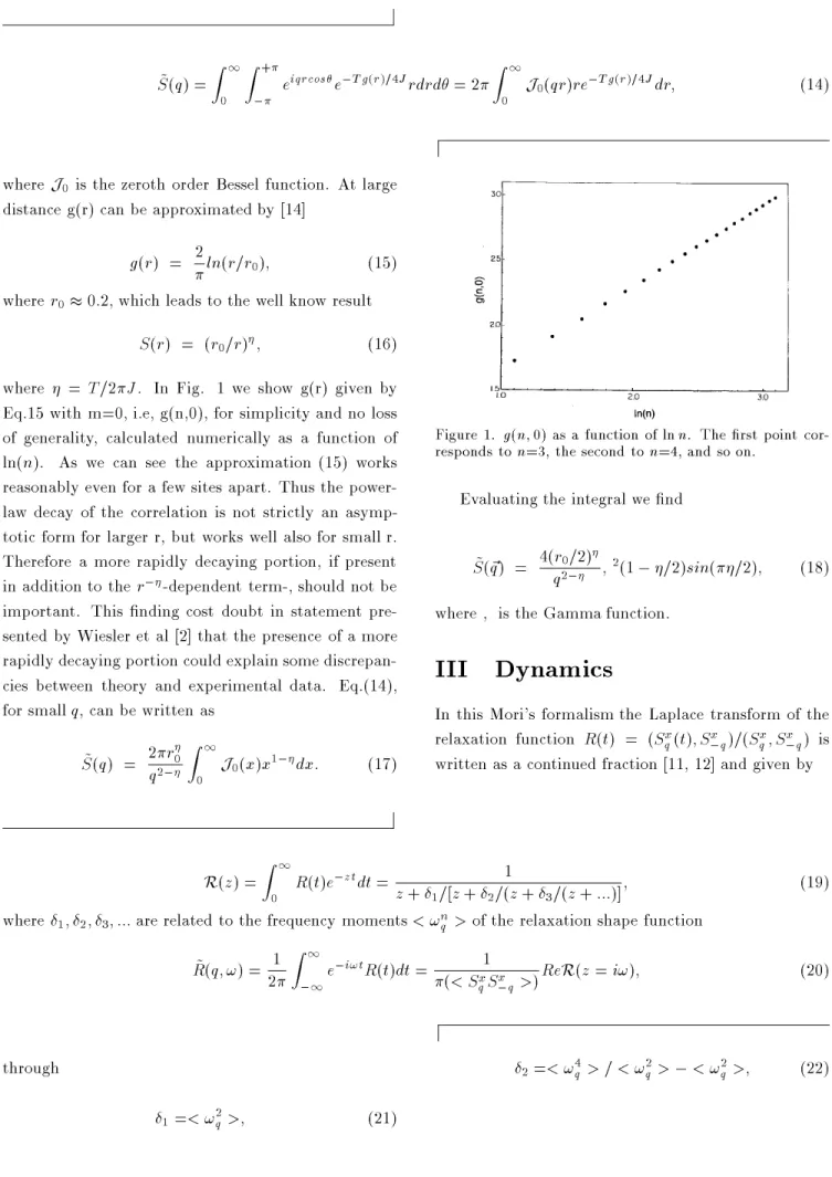
where = T=2 J. In Fig. 1 we show g(r) given by Eq.15 with m=0, i.e, g(n,0), for simplicity and no loss of generality, calculated numerically as a function of ln(n). As we can see the approximation (15) works reasonably even for a few sites apart. Thus the power-law decay of the correlation is not strictly an asymp-totic form for larger r, but works well also for small r. Therefore a more rapidly decaying portion, if present in addition to the r
,-dependent term-, should not be important. This nding cost doubt in statement pre-sented by Wiesler et al [2] that the presence of a more rapidly decaying portion could explain some discrepan-cies between theory and experimental data. Eq.(14), for smallq, can be written as
~
S(q) = 2 r
0 q
2, Z
1
0 J
0( x)x
1,
dx: (17)
Figure1. g (n;0)asafunction oflnn. Therstp oint cor-resp ondston=3,thesecondton=4,andsoon.
Evaluating the integral we nd ~
S(~q) = 4( r
0 =2)
q
2, ,
2(1
, =2)sin( =2); (18) where , is the Gamma function.
III Dynamics
In this Mori's formalism the Laplace transform of the relaxation function R(t) = (S
x q(
t);S x ,q)
=(S x q
;S x ,q) is written as a continued fraction [11, 12] and given by
c
R(z) = Z
1
0
R(t)e ,z t
dt=
1 z+
1 =[z+
2 =(z+
3
=(z+:::)]
; (19)
where 1
; 2
; 3
;:::are related to the frequency moments<! n q
>of the relaxation shape function ~
R(q ;!) = 12
Z 1
,1 e
,i! t
R(t)dt=
1 (<S
x q S
x ,q
>)
ReR(z=i!); (20)
d through
1=
<! 2 q
>; (21)
2=
<! 4 q
>=<! 2 q
>,<! 2 q
3= (
<! 6 q
>=<! 2 q
>,<! 4 q
> 2
=<! 2 q > 2) = 2 : (23) The dynamics structure factor, dened by
S(q ;!) = 12 Z 1 ,1 dte ,i! t <S x q(
t)S x ,q(0)
>; (24) is related to ~R(q ;!) by
S(q ;!) = q
!(1,e
, !),1~
R(q ;!); (25) where
qis the static susceptibility, which for a classical system is given by
q = <S x q S x ,q
>, where = 1=T and we have taken the Boltzman constant equals to the unity. Within the GA scheme the continued fraction (19) is truncated to the second stage, yielding[12, 15]
~
R(q ;!) = 1 1 2 a 2( !) [![!, 2 b 2( !)], 1] 2+ [
! 2 a 2( !)] 2 (26) with a 2 = (2 3) 1=2
exp(,! 2
=2
3) (27)
b 2 =
exp(,! 2 =2 3) ( 3 =2) 1=2 Z s 0 e x 2 dx (28)
s = ! =(2 3)
1=2 (29)
The integral in (28) was calculated numerically. The moments for Hamiltonian (1) can be calculated using standard procedure[12, 17]. The second moment has the exact relation with the two-spin correlation function
<! 2 q
>= 4JT <S x 0 S
x a
>=<S x q S x ,q > (30)
The fourth moment is expressed in terms of static cor-relation functions of four spin operators
<! 4 q
>= TM 4(
q)=<S x q S x ,q >; (31) with M 4= , X q ;p;t J q J p J t( <S x ,p S x ,q +t,k S y p+q +k > +<S
x ,p S x p+q +t S y ,q S y ,t >
,2<S x p+q +k S x ,q +t,k S y ,p S y ,t >
,<S y ,q S y ,t S y p+q +k S y ,p+t,K > +<S
y ,p S y ,q S y ,t S y p+q +t > +<S
y ,q S y p+q +k S z t,k S z ,p,t >
,<S y ,p S y ,q S z t,k S z p+q +k ,t
> +<S
y ,t S y ,p+t,k S z q +k S z p,q >
,<S z q +k S z p,q S z ,p,t S z t,k > +<S
x ,p S x p,q ,t S z q +k S z t,k > +<S
x ,p S x q +KT S z p,q S z t,k
>);: (32) where
J q = 2
J(cosq x +
cosq y)
: (33)
The estimation of the fourth and sixth moment at nite temperature is complicated and an approxima-tion is needed since there is no simple way in evaluating the four and six-spin correlation functions which are in-volved in the expression (32) and in a similarone for the sixth moment[16]. Let us, therefore, assume that the four and six-spin correlation functions may be approx-imated by a sum of products of appropriate pair cor-relation functions[17, 18, 19](mode-mode decoupling). Adopting this approximation we nd
c
M
4 =
,2[,32<S x 0 S
x 01
>(<(S x 0)
2
>+<S x 0 S
x 02
>+2<S x 0 S x 11 >) ,8<S
x 0 S
x 01
><(S z 0)
2
>+(<S x 0 S
x 01
>(18<S x 0 S x 12 > +3<S
x 0 S
x 03
>+43<S x 0 S
x 01
>)+<(S z 0) 2 > 2)( cosq x+ cosq y) ,<(S
z 0)
2
>(<(S x 0)
2
>+2<S x 0 S x 11 > +<S
x 0 S
x 02
>)(cos2q x+
cos2q y)]
(where the following notation has been used: 10-nearest neighbor, 02 and 11 next nearest neighbor, and 12 and 03 third nearest neighbor).
At very low temperatures, we obtain the asymptotic expression:
1 =
c 2
q 2
; (35)
2 = 8
t , c 2
q 2
t; (36)
which leads to
<! 4 q
> <! 2
>
2 (37)
<! 6 q
> <! 2
> 3
; (38)
where t=T/4J, and c=2J. AsT !0, 2
!0, ndR(q ;!) becomes a pair of delta functions at !=cq, the spin wave frequency.
IV Results
The structure ofS(q ;!) is ilustrated in Fig.2 and Fig.3 for T/J=0.05 and T/J=0.10 respectively and three val-ues of the wave vector q(in reciprocal lattice units). For the largest wave vector the collective mode dominates S(q ;!) but for small q there is considerable weight in S(q ;!) around ! = 0. The GA rounds o the diver-gence, found in former calculations[7, 8], of S(q ;!) at the spin wave frequency. The height of the resulting peaks will, however, diverge as q and ! tend to zero. The divergence described in [7, 8] appears because an arbitrary number of "spin waves" contribute coherently to the dynamic structure factor. This happens became in those calculations the linewidt of a single magnon was not taken into account [20]. The behavior of the spin-wave peak is best described by Fig.4, where we show the peak position !
q and the width at half-height , as a function of q for T/J=0.01, and Fig.5 where we show!
qand , as a function of T at
q= =10.
Figure 2. S(q ;! ) is show for three wave vectors, q = =10; =30; =40andforT/J=0.05.
Figure 3. S(q ;! ) is shown for three wave vectors, q = =10; =30; =40andforT/J=0.10.
As in similar calculations the use of the GA and 4-6-spin correlation function decoupling can be questioned. However the theory developed here should provide, at least qualitatively, a description of the dynamics of the two dimensional XY model at low temperatures, and be a rst step to a more elaborated calculation.
Figure 4. The spin-wave peak position!
q(a), and the
half-width at half-height ,(b) are show for T/J=0.01 and for
wave vector in the range 0:01q =0:1.
Figure 5. ! p(
a) and ,(b) are shown forq= =10, for
tem-peratures in the range 0:0T=J 0:02.
Acknowledgements
We wish to thank W. Oliveira and F.Takakura for their valuable discussion on the calculation for the sixth moment.
This work was partially supported by Con-selho Nacional de Desenvolvimento Cientco e Tec-nolologico(Brazil), and Capacitac~ao e Aperfeicoamento de Pessoal de Nvel Superior(Brazil).
References
[1] J.M. Kosterlitz, D.J. Thouless, J. Phys. C6, 1181
(1973).
[2] D.G. Wiesler, H. Zabel, S.M. Shapiro, Z. Phys. B93,
277 (1994), and references therein. [3] D.L. Huber, Phys. Rev. B26, 3758 (1982).
[4] D.P. Landau, R.W. Gerling, J. Magn. Mater. 104-107, 843 (1992).
[5] F.G. Mertens, A.R. Bishop, G.M. Wysin, C. Kawa-bata; Phys. Rev. Lett. 59, 117 (1987); Phys. Rev.
B39, 591 (1989).
[6] M.E. Gouvea, G.M. Wysin, A.R. Bishop, F.G. Mertens, Phys. Rev. B39, 11840 (1989).
[7] J. Villain; J. Phys. (Paris)35, 27 (1974).
[8] S.L. Menezes, A.S.T. Pires, M.E. Gouvea, Phys. Rev. B47, 12280 (1993).
[9] H.G. Evertz and D.P. Landau, Phys. Rev. B54, 12302
(1995); J.F.R. Costa and B.V. Costa, Phys. Rev. B54,
994 (1996).
[10] D.R. Nelson, D.S. Fisher, Phys. Rev. B16, 4945
(1977).
[11] H. Mori, Prog. Theor. Phys.34, 399 (1965).
[12] A.S.T. Pires, Helv. Phys. Acta61, 988 (1988).
[13] Y.J. Wang, M.R. Li, C.D. Gong, Phys. Rev. B56,
10982(1997).
[14] F. Spitzer, Principles of Random Walk. Princeton, Van Nostrand (1964).
[15] U. Balucani, V. Tognetti and R. Vallauri, Phys. Rev. A19, 177 (1979).
[16] Ph.D. thesis, \Estudo da estatica e din^amica de sis-temas de baixa dimensionalidade", Universidade Fed-eral de Minas Gerais (1998).
[17] S.W. Lovesey, R.A. Meserve, Phys. Rev. Lett.28, 614
(1971).
[18] S.W. Lovesey, R.A. Meserve, J. Phys. C6, 79 (1973).
[19] A.P. Young, B.S. Shastry, J. Phys. C15, 4547 (1982).
[20] M. Steiner, J. Villain and C.G. Windsor, Adv. Phys.