DOI: http://dx.doi.org/10.1590/2446-4740.07916 Volume 33, Number 1, p. 69-77, 2017
Introduction
Breast cancer is considered a major health problem in developed countries as well as in developing ones. This type of cancer is the second most frequent in the world and the most common among women. In 2017, an estimated 255,180 new cases of invasive breast cancer are expected to be diagnosed in the U.S. (Siegel et al., 2017).
In Brazil, breast cancer is still a disease with high levels of mortality due to late diagnosis, as the patient’s condition is too advanced. Among new cases of cancer, 57,960 cases of breast cancer were estimated for 2016, with 14,388 estimated deaths caused by such disease.
However, by diagnosing and treating in time, the prognosis of the disease can be good (Instituto..., 2016).
Tabár et al. (2005) support the theory that, before becoming systemic, breast cancer is limited to the breast for a variable time. Thus, the mammographic exam is the main resource for early diagnosis, inluencing directly on the mortality rate and even on the possibility of curative treatment. Women from ages 40 to 49 have a signiicant reduction of 15 to 20% in the mortality rate when submitted to such exam (Pisano et al., 2005; Senie et al., 1994).
Several studies in recent years have shown the relationship between the predominant type of tissue in the breast (breast density) and the risk of developing breast cancer (Heine et al., 2012; Kim et al., 2014; Llobet et al., 2014; Oliver et al., 2005; Petroudi et al., 2003). The risk of developing breast cancer is four to ive times bigger for women who had the predominance of ibroglandular tissue in the breast (dense breast) than for women with fatty breast (non-dense breast) (Oliver et al., 2005).
The amount of fat or glandular tissue which constitutes the breasts varies a lot among patients, and this is directly related to the biotype of each one, as well as to hormonal and genetic factors, among others, inluencing on how routine checkups are conducted (Riascos, 1999).
Breast density pattern characterization by histogram features and
texture descriptors
Pedro Cunha Carneiro
1*, Marcelo Lemos Nunes Franco
1, Ricardo de Lima Thomaz
1,
Ana Claudia Patrocinio
11Laboratory of Biomedical Engineering, Faculty of Electrical Engineering, Federal University of Uberlândia, Uberlândia, MG, Brazil.
Abstract Introduction: Breast cancer is the irst leading cause of death for women in Brazil as well as in most countries in the world. Due to the relation between the breast density and the risk of breast cancer, in medical practice, the
breast density classiication is merely visual and dependent on professional experience, making this task very
subjective. The purpose of this paper is to investigate image features based on histograms and Haralick texture
descriptors so as to separate mammographic images into categories of breast density using an Artiicial Neural
Network. Methods: We used 307 mammographic images from the INbreast digital database, extracting histogram features and texture descriptors of all mammograms and selecting them with the K-means technique. Then, these
groups of selected features were used as inputs of an Artiicial Neural Network to classify the images automatically
into the four categories reported by radiologists. Results: An average accuracy of 92.9% was obtained in a few
tests using only some of the Haralick texture descriptors. Also, the accuracy rate increased to 98.95% when texture
descriptors were mixed with some features based on a histogram. Conclusion: Texture descriptors have proven to be better than gray levels features at differentiating the breast densities in mammographic images. From this
paper, it was possible to automate the feature selection and the classiication with acceptable error rates since the
extraction of the features is suitable to the characteristics of the images involving the problem. Keywords Artiicial neural networks, Breast density, BI-RADS™, CAD, Digital mammography, Feature selection.
This is an Open Access article distributed under the terms of the Creative Commons Attribution License, which permits unrestricted use, distribution, and reproduction in any medium, provided the original work is properly cited.
How to cite this article: Carneiro PC, Franco MLN, Thomaz RL, Patrocinio AC. Breast density pattern characterization by histogram features and texture descriptors. Res Biomed Eng.2017; 33(1):69-77. DOI: 10.1590/2446-4740.07916.
*Corresponding author: Laboratory of Biomedical Engineering, Faculty of Electrical Engineering, Federal University of Uberlândia, Av. João Naves de Ávila, 2121, Santa Mônica, CEP 38408-100, Uberlândia, MG, Brazil. E-mail: [email protected]
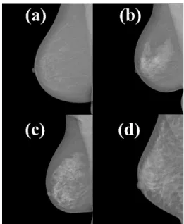
To evaluate the mammographic images, the American College of Radiology (ACR) has proposed the Breast Imaging Reporting and Data System (BI-RADS™) aiming at standardizing reports and mammogram characterization among doctors, residents and specialists in the ield (D’Orsi et al., 1998). In this way, four categories were created to classify the breast according to its density:
• Category a: the breast is predominantly adipose (fat);
• Category b: there are scattered areas of ibroglandular density;
• Category c: the breast is heterogeneously dense, which may obscure small masses;
• Category d: the breast is extremely dense, which lowers the sensitivity of mammography. In the old BI-RADS™ edition, breast density was divided into categories 1 to 4. In the new edition, breast composition categories are ‘a’, ‘b’, ‘c’ or ‘d’. The current ‘category a’ corresponds to the former ‘category 1’, the ‘category b’ to the former ‘category 2’ and so on (Mercado, 2014). Using percentages is discouraged because a better indicator of the risk of cancer would be the amount of ibroglandular tissue able to obscure a mass rather than the percentage of the predominant tissue in the breast (D’Orsi et al., 1998; Mercado, 2014).
Taking into account that the difference in intensity and texture among images from different categories is signiicant, the use of features based on a histogram and Haralick texture descriptors has constantly been studied in the literature (Kallenberg et al., 2011; Keller et al., 2012; Manduca et al., 2009; Oliver et al., 2008; 2010; Petroudi et al., 2003; Riascos, 1999). However, as the classiication of breast density is very subjective even for experts, in many cases, the category 2 (‘b’) is mistaken for the category 3 (‘c’) and vice versa.
Due to that, it is important to come up with a tool that can help classifying images by breast density, since the assessment of dense breasts is highly complex, making it dificult to detect lesions. In order to do so, different combinations of features extracted from mammograms were evaluated, and after they had been selected, we check what set and type of features can better classify this kind of image.
The contrast pattern in screen-ilm images provided a contrast characterization of breast density primarily by the variation in pixel intensities. However, this visual assessment has changed since digital imaging due to preprocessing algorithms, in which the breast density determination includes visual texture characteristics, and not only the gray level variation, changing the assessment paradigm. Thus, the approach of this paper is that mammograms classiied into different categories for breast density are represented by different tissues
with various characteristics. Therefore, each pattern density should present distinct characteristic each other.
The main goal of this work is to extract features of digital mammographic images (based on histogram and Haralick descriptors), select the best of them using K-means, and evaluate what type of features best characterizes digital mammographic images. With the best selected characteristics, images should be classiied in the four BI-RADS™ categories of breast density using an artiicial neural network (ANN) as a pattern classiication method.
Methods
The steps taken to develop this paper are described next.
Dataset
We used 307 mammographic images from the digital INbreast database (Moreira et al., 2012), along with the radiologists’ classiication using the four categories of breast density. As the new BI-RADS™ update is recent, the reports provided by the staff for this database was based on its previous edition. Nevertheless, this does not change the primary objective of this paper.
Of these 307 images used, 103 belong to category 1 (fatty breast), 104 mammograms belong to category 2, 73 to category 3, and the 27 remaining images belong to category 4 (dense breast). Figure 1 presents examples of the dataset used to exemplify the four categories of breast density based on the BI-RADS™.
The mammographic breast density classiication is a visual process, thus, there is a high degree of subjectivity, and it is strongly dependent on the professional’s experience. In this work the reports made by radiologists were considered the gold standard.
These images are in the DICOM format (Digital Imaging and Communications in Medicine), 12 bits per pixel, 3328 × 4084 or 2560 × 3328 pixels, depending on the size of the patient’s breast. They were obtained with the same equipment, a MammoNovation Siemens FFDM (Full Field Digital Mammography), and in this work both mediolateral oblique (MLO) and craniocaudal (CC) images were processed.
Feature extraction
In literature, some studies which classify mammograms into breast density using features based on histograms were proposed (Karssemeijer, 1998; Wang et al., 2003; Zhou et al., 2001). However, our experience has shown that using only features based on histograms are not suficient for classifying the images because of the post-processing algorithm used in digital mammography.
In screen-ilm mammography used years ago, the four categories of breast density could be identiied by analyzing the gray levels (histogram), in which category ‘a’ (fatty breast) had a lower gray level average (GLA) of pixels of the histogram compared to images in category ‘d’ (dense breast). This intensity difference occurs because most soft tissues, such as the adipose tissue, allow the radiation to get through more easily. As a result, mammograms with a predominance of fat appear darker than the images with a ibroglandular tissue because this type of tissue absorbs much of the radiation.
In digital mammography systems, each manufacturer has its own post-processing algorithm with a contrast window function. Hence, there is a variation in the gray level of the images (Mousa et al., 2014). Thus, analyzing only features extracted from histograms can confuse the classiication, where dense breast images from category ‘d’ can present a lower GLA when compared to the other categories of breast density. This variation contradicts the logic presented in the screen-ilm mammography.
For this reason, in this paper, we decided to combine features extracted from histograms and Haralick texture descriptors, since, in digital images, texture variation occurs more clearly than the variation of gray levels. We extracted nine features from histograms and 14 Haralick texture descriptors (Gonzalez and Woods, 2007; Haralick et al., 1973).
Before the feature extraction, the preprocessing step used in this work was the removal of the background from the image. Therefore, we assure that the extracted features correspond to the entire glandular portion of the mammographic image.
The features extracted from histograms were: gray level average (GLA), value of intensity of the highest peak of the histogram (mode), value of the lowest intensity of the histogram, value of the highest intensity of the histogram, percentage of the highest intensity compared to the maximum possible intensity, subtraction of the average to the lowest value, the highest pixel value of the image subtracted from its average, number of pixels higher than the peak, and gradient (subtraction of the highest intensity to the lowest intensity).
The image texture contains information about the spatial distribution of intensity variations within a range of values (Gonzalez and Woods, 2007) and the texture features used in this work were the Haralick texture descriptors (Haralick et al., 1973). These descriptors use the gray level co-occurrence matrix (SGLD - Spatial Gray- Level Dependence) to calculate the probability of combined occurrence of direction and distance between pairs of pixels with similar intensity values, separated by a distance (d) in an angle (θ).
The co-occurrence matrix takes into account the relationship between two pixels at a time, the irst being called the reference pixel, and the second, the neighboring pixel. In this paper, we produced the texture features from the average of the value obtained for each of the four angles (0º, 45º, 90º, 135º) with distance equal to 1 (d=1) (Haralick et al., 1973; Horsthemke and Raicu, 2007).
A set of 14 Haralick descriptors were implemented, namely: energy or uniformity; contrast; correlation; variance; inverse difference moment; sum average; sum variance; sum entropy; entropy; difference variance; difference entropy; information measure of correlation 1; information measure of correlation 2; and maximum correlation coeficient.
For each image, we extracted nine features from the histogram and 14 Haralick texture descriptors. We calculate average, and standard deviations for all the 23 features of images in the same category, and the values obtained were compared in each of the categories.
Feature selection
The feature selection is a step of the data preprocessing phase. The purpose of this step is to choose one or more subsets of features which reduce the complexity of the database in addition to reducing the processing and amount of variables to be analyzed. With this size reduction, the processing time becomes smaller and unnecessary features are removed from the classiication stage, avoiding features that may cause confusion in the inal results.
The K-means is a non-hierarchical heuristic of clustering which aims at minimizing the distance from the elements to a cluster of k centers given by χ={x1,x2,...,xk}
in an iterative way. The distance between a pi point and a set of clusters, given by d(pi,χ), is deined as being the distance from the point to the nearest center. We used k equal to 4, corresponding to four clusters, one for each class of breast density. The equation of K-means (1) is presented below, where ||xi(j) - c
j||
2 is a chosen distance
measure between a data point xi(j) and the cluster center c j:
1 1 2
− −
=∑ ∑k n j−
i j
j i
J x c (1)
All the 23 features were tested individually in the K-means technique. The features that obtained more than 60% of hit rate in the feature selection classiication were combined simultaneously in the K-means technique and, with the best results obtained, we created a subset of features to be used in the classiication technique (ANN) as shown in the Results Section.
Density classiication
After the extraction and the selection of the features, we used an ANN as a pattern classiication method (Kovács, 1996; Patterson, 1998). The main goal was to classify the images into the four existing categories of breast density, as well as to verify if these images were classiied into the correct category.
The ANN was implemented using the MATLAB neural network toolbox (Beale et al., 2015). Among the many existing artiicial neural networks, the supervised feedforward neural network model with the backpropagation learning algorithm was chosen to be used in this paper.
A backpropagation algorithm seeks iteratively to ind the minimum difference between desired outputs (DO) and outputs (O) obtained by the neural network with the least number of errors (E). Thus, the error in the output layer is calculated and backpropagated in the opposite direction (output → input). The weights are, then, adjusted between the layers through the backpropagation in each iteration (Beale et al., 2015; Haykin, 2004; Patterson, 1998; Rumelhart et al., 1988).
The training function used was ‘traingdx’ which means a gradient descent with momentum and an adaptive learning rate backpropagation. In this network, the training function updates weight and bias values according to a gradient descent momentum and an adaptive learning rate (Beale et al., 2015).
Backpropagation is used to calculate derivatives (Equation 2) of performance (perf) on the weight and bias variables X (Beale et al., 2015). Each variable is adjusted according to a gradient descent with momentum, where
mc is the momentum constant, dXprev is the previous change to the weight and bias, lr is the learning rate:
( )
= × + × ×
dperf
dx mx dxprev lr mc
dx (2)
For each epoch, if performance decreases toward the goal, then the learning rate is increased by a factor called learning rate increase. If performance increases
by more than the parameter of maximum performance
increase, the learning rate is adjusted by the factor called
learning rate decrease and the change that increased the performance is not made.
The training stops when any of these conditions occurs: the maximum number of epochs (repetitions) is reached; the maximum amount of time is exceeded; performance is minimized to the goal; the performance gradient falls below the minimum performance gradient, and validation performance increases more than the maximum validation failures since the last time it decreased (when using validation).
In this model of neural network, the user can change and vary the coniguration, such as the number of neurons in the input and hidden layer, the activation function of each of this layers, the number of epochs, the minimum performance gradient, and the maximum validation failures.
The number of neurons in the input layer corresponds to the number of features that were being analyzed. Only one hidden layer was used, and the number of neurons in this layer was tested one to three times greater than the number of neurons in the input layer (one by one) so, if the set of features analyzed was 8, the minimum number of neurons tested was 8, and the maximum, 24. The number of neurons in the output layer is ixed and equal to 2 (in this case). This number of neurons means that the output was given in binary values (Islam et al., 2010; Rouhi et al., 2015).
The number of epochs was tested changing its value from 100,000 to 200,000 epochs, the minimum performance gradient was set as 10-6, and the maximum
validation failures were tested, and the values ranged from 10,000 to 100,000.
We produced four groups of features which were separately tested in the neural network with different conigurations according to the feature selection obtained by the K-means method. Once the best results were obtained, the neural network coniguration, including the numbers of neurons and activation functions, was saved, and each neural network (4 ANNs, one for each group of selected features, presented in Results Section) was trained ten times. The inal result for the classiier was the average of these ten training sessions using such coniguration.
For categories 1, 2 and 3, 51 images were used for training and, for category 4, we used 19 images in the training group. The training group has a part of images for the network training, and another part is separated for test and validation. On the other hand, the test group, which was randomly generated, is tested independently after the training, allowing us to verify the performance of the Artiicial Neural Network.
Of the 307 images, we used 172 images in the training group and 135 images in the test group. The number (n) of images for each class of breast density assigned to the training and test group are shown in Table 1. For all the ANNs, the same set of samples, i.e., the same number of images for each class of breast density was used, in accordance with Table 1.
Results
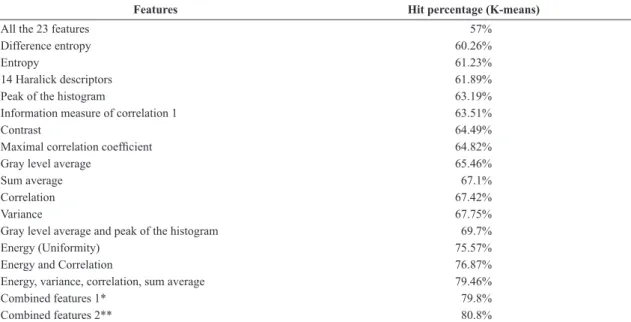
Table 2 presents the results obtained through feature selection by using the K-means technique. The more accurate the rate of a feature is, the better it is to classify the images, and thus, probably it will be a useful feature to be used in the ANN.
The result of the K-means technique for all the 23 features (57% of accuracy) showed and motivated
the importance of the feature selection. Even so, one of the artiicial neural network tested was with all the 23 features as input (ANN 4) to compare with the ANNs that a set of selected features were used as input.
In general, when the features were not combined among themselves, it became apparent that the texture descriptors showed better results compared to the one extracted from the histogram. The results ranged from 60.26% (difference entropy) to 75.57% (energy or uniformity) of hit accuracy. For the intensity features, the best individual results were for GLA and peak of the histogram, with 65.46% and 63.19% of accuracy rate, respectively.
After testing the features individually, we decided to combine two or more features (hit rate greater than 60%), trying to produce better results for the K-means. In some cases, this combination was not successful, such as when we used only features extracted from the histogram, resulting in a small percentage hit (33%), far lower than the accuracy of the 14 Haralick descriptors.
The best results for K-means, i.e., the features which proved to be the best for clustering images into the four categories of breast density, were those combined and applied simultaneously, as shown in Table 2: ‘Combined Features 1’ and ‘Combined Features 2’.
Table 1. The number of images for each class in the training and test groups of the artiicial neural network.
Group n(Class 1) n(Class 2) n(Class 3) n(Class 4)
Training 51 51 51 19
Test 52 53 22 08
Total 103 104 73 27
Table 2. Feature selection: hit percentage of some features using K-means.
Features Hit percentage (K-means)
All the 23 features 57%
Difference entropy 60.26%
Entropy 61.23%
14 Haralick descriptors 61.89%
Peak of the histogram 63.19%
Information measure of correlation 1 63.51%
Contrast 64.49%
Maximal correlation coeficient 64.82%
Gray level average 65.46%
Sum average 67.1%
Correlation 67.42%
Variance 67.75%
Gray level average and peak of the histogram 69.7%
Energy (Uniformity) 75.57%
Energy and Correlation 76.87%
Energy, variance, correlation, sum average 79.46%
Combined features 1* 79.8%
Combined features 2** 80.8%
‘Combined Features 1’ resulted in 79.8% accuracy, being composed of the following Haralick descriptors: energy, variance, correlation and sum average, as well as the features extracted from the histogram: GLA (gray level average), peak of the histogram, gradient and the highest pixel value of the image subtracted from its average.
The best result was with the ‘Combined Features 2’ with 80.8% of hit rate. This set of features is a combination of Haralick descriptors and intensity features too, such as energy, variance, correlation, sum average, GLA and peak of the histogram.
From the results of the feature selection, we proposed four test groups (ANNs) formed by sets of features (ANN 1 comprises the ‘Combined Features 1’ as input, ANN 2 comprises the ‘Combined Features 2’ as input, ANN 3 is formed only by texture descriptors with 60% or more of hit rate as input, and the ANN 4 comprises the 23 extracted features):
• Input features set for ANN 1: energy, variance, correlation, sum average, GLA, peak of the histogram, gradient and the highest pixel of the image subtracted from its average;
• Input features set for ANN 2: energy, variance, correlation, sum average, GLA and peak of the histogram;
• Input features set for ANN 3: energy, variance, correlation, sum average, difference entropy, entropy, information measures of correlation 1 and 2, contrast and maximal correlation coeficient;
• Input features set for ANN 4: nine features from histograms and 14 Haralick texture descriptors combined.
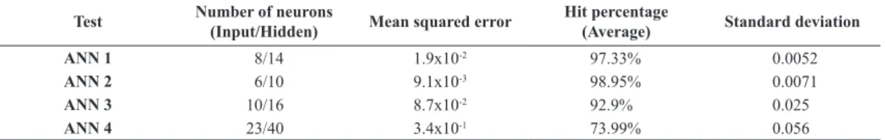
Table 3 shows the number of neurons used in the input and hidden layers for each test, the mean squared error (MSE), hit percentage average for the ANN and the standard deviation from the ten training and tests. These results consist of the average of ten training sessions and tests of the ANN with the best coniguration. The best results were obtained using log-sigmoid as an activation function for all the ANNs.
From Table 3, the best accuracy was obtained in ANN 2 with approximately 98.95%, on average, of hit percentage. The number of neurons used in the input
and hidden layer for this test was 6 and 10, respectively, and the mean squared error equals to 9.1.10-3. The best
coniguration for ANN 1 was with eight neurons in the input layer and 14 on the hidden layer. These settings obtained 97.33% of hit percentage and a mean squared error of 1.9.10-2. When, for ANN3, ten features and
16 neurons were used in the hidden layer, the hit percentage obtained was 92.9% of classiication.
For the ANN 4, that one with the worst classiication result, the classiication obtained 73.99%, on average, of hit accuracy. This way, the mean squared error calculated was too high (3.4.10-1), indicating the increased ANN’s
degree of confusion. Using all the 23 extracted features as input, the best coniguration had 40 neurons in the hidden layer.
During the ten training sessions and tests, the best result obtained for ANN 1 was 97.78% of hit percentage and the worst, 96.29%. ANN 2 achieved 99.26% of hit accuracy (the best result for this ANN), and the worst result was 97.03% of hit accuracy. For ANN 3, the best result achieved a success rate of 95.55%, and the worst result was 88.15% of hit rate. The best and worst result obtained for ANN 4, during the ten training sessions and tests, was 76.29% and 70.37% of hit percentage, respectively.
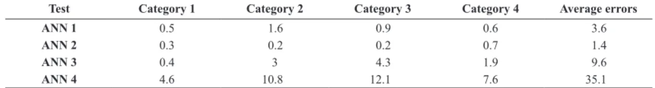
Another analysis conducted is about the number of errors made by the ANN algorithm. In other words, the number of confusion/mistakes the algorithm made classifying a certain image out of its original category were counted.
During the ten training sessions and tests, for ANN 1, 36 mistakes were made in total, for ANN 2, 14 mistakes, for ANN 3, 96 mistakes, and for ANN 4, 351 mistakes. This number of errors indicates that, for each training, on average, the Artiicial Neural Network classiies 3, 1.4, 9.6, and 35.1 images wrongly for ANN 1, ANN 2, ANN 3, and ANN 4, respectively. Table 4 summarizes these results.
The best results for ANN 1, ANN 2, ANN 3, and ANN 4 generated three, one, six, and 32 mistakes, respectively. Most of the errors were related to the inversion of category 2 to category 3 of breast density, causing two out of the three mistakes for ANN 1, four out of the six mistakes for ANN 3, and 11 out of the 32 mistakes for ANN 4. For the ANN 2, the only mistake was classifying as category 3 what was, in fact, category 4.
Table 3. Hit percentage of the Artiicial Neural Network.
Test Number of neurons
(Input/Hidden) Mean squared error
Hit percentage
(Average) Standard deviation
ANN 1 8/14 1.9x10⁻² 97.33% 0.0052
ANN 2 6/10 9.1x10⁻³ 98.95% 0.0071
ANN 3 10/16 8.7x10⁻² 92.9% 0.025
Discussion
The K-means technique has revealed itself as a good feature selection method, allowing us to choose the most relevant features from it, thus, reducing probable characteristics that would cause confusion in the ANN. In addition, without the feature selection, i.e., when we used all the 23 features, the low accuracy justiies the selection of a set of features, trying to improve the computational cost and the classiication.
Fewer images from the category 4 (dense breast) of breast density could lead to problems for the neural network classiication, e.g., overitting, misclassiication or underestimating the category samples. Thus, for trying to avoid these problems, we cross-validated the network 10 times, on which random groups for training and testing were generated for evaluation.
The results (hit accuracy) obtained using Haralick texture descriptors were higher than the features extracted from the histogram. This is caused because the digital images distinguish themselves more in texture rather than in intensity of gray level, as a result of post-processing. Images with a dominance of fat tissue should display lower intensity compared to images with a dominance of ibroglandular tissue, but this was not what the indings revealed. Nevertheless, the difference in texture between these types of tissue has become more evident due to the greater variation in intensity within a range of values.
The features based on the histograms have revealed a high variance in the same category, which could be explained by the presence of nodular lesions in the images, changing the level of intensity of pixels between them and making it harder to classify from these features.
Analyzing Table 2, it is possible to verify that the best results are obtained when more than one feature is used concurrently with the technique of feature selection. Nonetheless, as a feature is added, the group of features does not necessarily get better. This effect, known as dimensionality curse, occurred when the 23 features analyzed simultaneously produce worse results that when a smaller number of features are analyzed.
ANN 2 has scored the best result of the neural network with only 14 mistakes during the ten training sessions and tests of the network. On average, 98.95% of the images were classiied correctly in their category.
The ‘energy’ feature indicates homogeneity, which means more homogeneous textures, such as images
from category 4. These images have a higher energy compared to the images of the other categories of breast density. ‘Variance’, ‘correlation’ and ‘sum average’ are related to the image background. The irst denotes the intensity variation of the image background, the second is an indicator of an implicit structure in the texture, and the last, ‘sum average’ descriptor, is an average of the image background pixels. ‘GLA’ and ‘peak of the histogram’ indicate the gray level average, in which darker images tend to have a lower GLA value, and the histogram mode, respectively.
For ANN 2 the higher confusion was when classifying images of category 4. This confusion is probably due to the lower number (8) of images tested, as there were few cases of such category in the database to be used. For ANN 1, ANN 3, and ANN 4 the vast majority of the mistakes were in the intermediate categories, 2 and 3 of the density category, due to the similarity of texture from images of such category.
However, the intrinsic subjectivity of the mammographic classiication process by categories of density makes the task even more dificult and subjected to results with a higher level of confusion. Through the use of a clustering technique, it is possible to develop an automatic system to aid this task with an acceptable number of mistakes since the extraction of features is adequate to the characteristics of the image that involves the problem.
Comparing our study with others in the literature, Mustra et al. (2012) extracted texture features for breast density classiication using k-nearest neighbor’s (k-NN) algorithm achieving 76.4% of hit rate (Mustra et al., 2012). Oliver et al. (2005) classiied 300 mammographic images using k-NN with 67% of accuracy, extracting texture and morphological features (Oliver et al., 2005). Wang et al. (2003) achieve 71% of hit rate using an ANN for the classiication of 195 mammographic images in four categories of breast density (Wang et al., 2003).
Our work contributes to the classification by breast density, indicating that the images could be differentiated more by texture descriptors than by gray levels (histogram). With the use of an Artiicial Neural Network, and a method of feature selection, 98.95% of the images were classiied correctly within its category. From this method it was possible to automate this task, aiding radiologists in the report of the categories of breast density and possibly increasing the detection of breast cancers.
Table 4. Average of the number of mistakes and errors made by the Artiicial Neural Network for each category of breast density.
Test Category 1 Category 2 Category 3 Category 4 Average errors
ANN 1 0.5 1.6 0.9 0.6 3.6
ANN 2 0.3 0.2 0.2 0.7 1.4
ANN 3 0.4 3 4.3 1.9 9.6
The next steps of the project are: implementing an image segmentation technique, with the removal of the pectoral muscle; expanding the database, adding more images of categories 3 and 4; and also including this automatic model in a computer-aided diagnosis system, which is being developed by this research group.
Acknowledgements
We would like to thank the Breast Research Group, INESC Porto, Portugal, for providing the images and CAPES for the inancial support.
References
Beale MH, Hagan MT, Demuth HB. Neural network toolbox: users guide. Natick: Mathworks; 2015.
D’Orsi C, Basset L, Feig S. Illustrated breast imaging reporting and data system American College of Radiology. Reston: American College of Radiology; 1998.
Gonzalez RC, Woods RE. Digital image processing. 3th ed. Upper Saddle River: Prentice Hall; 2007.
Haralick RM, Shanmugam K, Dinstein I. Textural features for image classification. IEEE Transactions on Systems, Man, and Cybernetics. 1973; SMC-3(6):610-21. http://dx.doi.org/10.1109/ TSMC.1973.4309314.
Hartigan JA, Wong MA. Algorithm AS 136: a K-means clustering algorithm. Applied Statistics. 1979; 28(1):100-8. http://dx.doi.org/10.2307/2346830.
Haykin S. Neural networks: a comprehensive foundation. 2nd ed. Englewoods Cliffs: Prentice Hall; 2004.
Heine JJ, Scott CG, Sellers TA, Brandt KR, Serie DJ, Wu FF, Morton MJ, Schueler BA, Couch FJ, Olson JE, Pankratz VS, Vachon CM. A novel automated mammographic density measure and breast cancer risk. Journal of the National Cancer Institute. 2012; 104(13):1028-37. PMid:22761274. http:// dx.doi.org/10.1093/jnci/djs254.
Horsthemke WH, Raicu DS. Organ analysis and classification using principal component and linear discriminant analysis. In: Pluim JPW, Reinhardt JM, editors. Medical Imaging: Proceedings of SPIE: International Society for Optics and Photonics; 2007 Mar 5; San Diego, US. Bellingham: SPIE; 2007. p. 65124A-11.
Instituto Nacional de Câncer. Estimativa 2016: Incidência de câncer no Brasil. Rio de Janeiro: INCA; 2016.
Islam MJ, Ahmadi M, Sid-Ahmed MA. An efficient automatic mass classification method in digitized mammograms using artificial neural network. Int J Artif Intell Appl. 2010; 1(3):1-13. http://dx.doi.org/10.5121/ijaia.2010.1301.
Kallenberg MGJ, Lokate M, van Gils CH, Karssemeijer N. Automatic breast density segmentation: an integration of different approaches. Physics in Medicine and Biology. 2011; 56(9):2715-29. PMid:21464531. http://dx.doi.org/10.1088/0031-9155/56/9/005.
Karssemeijer N. Automated classification of parenchymal patterns in mammograms. Physics in Medicine and Biology. 1998;
43(2):365-78. PMid:9509532. http://dx.doi.org/10.1088/0031-9155/43/2/011.
Keller BM, Nathan DL, Wang Y, Zheng Y, Gee JC, Conant EF, Kontos D. Estimation of breast percent density in raw and processed full field digital mammography images via adaptive fuzzy c-means clustering and support vector machine segmentation. Medical Physics. 2012; 39(8):4903-17. PMid:22894417. http:// dx.doi.org/10.1118/1.4736530.
Kim Y, Hong BW, Kim SJ, Kim JH. A population-based tissue probability map-driven level set method for fully automated mammographic density estimations. Medical Physics. 2014; 41(7):71905. PMid:24989383. http://dx.doi.org/10.1118/1.4881525.
Kovács ZL. Redes neurais artificiais. 2nd ed. São Paulo: Acadêmica; 1996.
Llobet R, Pollán M, Antón J, Miranda-García J, Casals M, Martínez I, Ruiz-Perales F, Pérez-Gómez B, Salas-Trejo D, Pérez-Cortés JC. Semi-automated and fully automated mammographic density measurement and breast cancer risk prediction. Computer Methods and Programs in Biomedicine. 2014; 116(2):105-15. PMid:24636804. http://dx.doi.org/10.1016/j. cmpb.2014.01.021.
Manduca A, Carston MJ, Heine JJ, Scott CG, Pankratz VS, Brandt KR, Sellers TA, Vachon CM, Cerhan JR. Texture features from mammographic images and risk of breast cancer. Cancer Epidemiology, Biomarkers & Prevention. 2009; 18(3):837-45. PMid:19258482. http://dx.doi.org/10.1158/1055-9965. EPI-08-0631.
Mercado CL. BI-RADS Update. Radiologic Clinics of North America. 2014; 52(3):481-7. PMid:24792650. http://dx.doi. org/10.1016/j.rcl.2014.02.008.
Moreira IC, Amaral I, Domingues I, Cardoso A, Cardoso MJ, Cardoso JS. INbreast: toward a full-field digital mammographic database. Academic Radiology. 2012; 19(2):236-48. PMid:22078258. http://dx.doi.org/10.1016/j.acra.2011.09.014.
Mousa DS, Mello-Thoms C, Ryan EA, Lee WB, Pietrzyk MW, Reed WM, et al. Mammographic density and cancer detection: does digital imaging challenge our current understanding. Academic Radiology. 2014; 21(11):1377-85. PMid:25097013. http://dx.doi.org/10.1016/j.acra.2014.06.004.
Mustra M, Grgić M, Delač K. Breast density classification
using multiple feature selection. Autom J Control Meas Electron Comput Commun. 2012; 53(4):362-72. http://dx.doi. org/10.7305/automatika.53-4.281.
Oliver A, Freixenet J, Marti R, Pont J, Perez E, Denton ERE, Zwiggelaar R. A novel breast tissue density classification methodology. IEEE Transactions on Information Technology in Biomedicine. 2008; 12(1):55-65. PMid:18270037. http:// dx.doi.org/10.1109/TITB.2007.903514.
Oliver A, Freixenet J, Zwiggelaar R. Automatic classification of breast density. In: Image Processing: Proceedings of IEEE International Conference; 2005 Sept 11-14; Genova, Italy. USA: IEEE; 2005. p. II-1258. http://dx.doi.org/10.1109/ ICIP.2005.1530291.
Patterson DW. Artificial neural networks: theory and applications. 1st ed. Upper Saddle River: Prentice Hall; 1998.
Petroudi S, Kadir T, Brady M. Automatic classification of mammographic parenchymal patterns: a statistical approach. In: Engineering in Medicine and Biology Society: Proceedings of the 25th Annual International Conference of the IEEE; 2003 Sept 17-21; Cancún, Mexico. USA: IEEE; 2003. p. 798-801.
Pisano ED, Gatsonis C, Hendrick E, Yaffe M, Baum JK, Acharyya S, Conant EF, Fajardo LL, Bassett L, D’Orsi C, Jong R, Rebner M. Diagnostic performance of digital versus film mammography for breast-cancer screening. The New England Journal of Medicine. 2005; 353(17):1773-83. PMid:16169887. http://dx.doi.org/10.1056/NEJMoa052911.
Riascos A. Vertical mammaplasty for breast reduction. Aesthetic Plastic Surgery. 1999; 23(3):213-7. PMid:10384021. http:// dx.doi.org/10.1007/s002669900270.
Rouhi R, Jafari M, Kasaei S, Keshavarzian P. Benign and malignant breast tumors classification based on region growing and CNN segmentation. Expert Systems with Applications. 2015; 42(3):990-1002. http://dx.doi.org/10.1016/j.eswa.2014.09.020.
Rumelhart DE, Hinton GE, Williams RJ. Learning representations by back-propagating errors. Nature. 1988; 323(6088):533-8. http://dx.doi.org/10.1038/323533a0.
Senie RT, Lesser M, Kinne DW, Rosen PP. Method of tumor detection influences disease-free survival of women with breast carcinoma. Cancer. 1994; 73(6):1666-72. PMid:8156494. http:// dx.doi.org/10.1002/1097-0142(19940315)73:6<1666::AID-CNCR2820730619>3.0.CO;2-E.
Siegel RL, Miller KD, Jemal A. Cancer statistics, 2017. CA: a Cancer Journal for Clinicians. 2017; 67(1):7-30. PMid:28055103. http://dx.doi.org/10.3322/caac.21387.
Tabár L, Tot T, Dean PB. Breast Cancer: the art and science of early detection with mammography: perception, interpretation, histopathologic correlation. Stuttgart: Thieme; 2005. p. 405-38.
Wang XH, Good WF, Chapman BE, Chang Y-H, Poller WR, Chang TS, Hardesty LA. Automated assessment of the composition of breast tissue revealed on tissue-thickness-corrected mammography. AJR. American Journal of Roentgenology. 2003; 180(1):257-62. PMid:12490516. http://dx.doi.org/10.2214/ ajr.180.1.1800257.