DOI: http://dx.doi.org/10.1590/2446-4740.03316 Volume 33, Number 1, p. 11-20, 2017
Introduction
Cardiovascular diseases (CVD) have been the focus of research in recent years due to its high mortality rate. It is estimated that 17.5 million people died of CVD in 2012, from which 7.4 million were due to coronary heart disease (CHD) (World..., 2014). CHD is a cardiac disease in which plaque builds up inside the coronary arteries consequently narrowing them and reducing the blood low to the heart muscle. Depending on the occlusion degree it can cause many complications such as stroke, heart attack and death (Cohen and Hasselbring, 2007).
One of the most common procedures used to treat CHD is the insertion of stent structures in the coronary artery. They are inserted through a catheter and expanded at the site of the blockage, resetting the vessel size of the stented segment. Even though the procedure shows good results, restenosis may still occur, showing great
importance in monitoring the vessel’s status (Mittal, 2005). The most recent technology used for that purpose is the Frequency Domain Intravascular Optical Coherence Tomography (FD-IOCT). It produces high-resolution images of the vessel wall by both emitting light and recording the reflection through a catheter while simultaneously rotating it and pulling it back along the artery (Bezerra et al., 2009).
To evaluate quantitatively the accumulated tissue over the stent (neointimal tissue) it is necessary to segment the lumen and stented area, which is usually done manually by a specialist. To avoid this time consuming task and accelerate the process some potential applications have been developed.
Exploring the FD-IOCT technique, Tsantis et al. (2012) developed a method to automatically segment lumen and stent of femural arteries. It identiies the lumen through a technique based on Markov Model (Li, 1995), and later detects stent struts using Wavelet Transform (Mallat and Hwang, 1992) and iltering with intensity, energy and shadow features. Mandelias et al. (2013) created an application with graphical interface focused on clinical use. Also focusing on femoral arteries, it uses algorithms based on fuzzy C-means clustering (Bezdek et al., 1984) and Wavelet Transform to extract the lumen border and stent struts’ location. Ughi et al. (2012) presented a semi-automatic algorithm where the user performs an initial parameter calibration for coronary artery images, and later automatically identiies
Approaches to segment stent area from Intravascular Optical Coherence
Tomography
Veronica Meyer Gaiarsa
1*, Diego Cardenas
1, Sergio Shiguemi Furuie
11Biomedical Engineering Laboratory, University of Sao Paulo – USP, São Paulo, SP, Brazil.
Abstract Introduction: Cardiovascular diseases (CVD) have been the focus of research in recent years due to its high
mortality rate. It is estimated that 17.5 million people died of CVD in 2012, from which 7.4 million were due to coronary heart disease (CHD). In order to monitor CHD patients and avoid waste of specialists’ time, this study proposes the development of a method that segments the area contained by stent struts from Frequency Domain Intravascular Optical Coherence Tomography (the latest technology to view vessels internally) of coronary arteries.
Methods: The novelty of this study is to ind areas comprised by stent struts using two optimal strategies that are
robust even with false positives and false negatives detection of stent struts. The irst one uses an ellipse itting algorithm and the other uses a cylinder itting algorithm. Results: Both strategies obtained similar accuracy results close to 98% of true positives, but the cylinder technique showed a run time of at least 50 times higher than the ellipse technique. Conclusion: The methods were executed on 443 images with different characteristics showing robustness and usefulness in the medical area.
Keywords Stent, IOCT-FD, Segmentation, Cylinder itting, Moving window iterative ellipses.
This is an Open Access article distributed under the terms of the Creative Commons Attribution License, which permits unrestricted use, distribution, and reproduction in any medium, provided the original work is properly cited.
How to cite this article: Gaiarsa VM, Cardenas D, Furuie SS. Approaches to segment stent area from Intravascular Optical Coherence Tomography. Res Biomed Eng.2017; 33(1):11-20. DOI: 10.1590/2446-4740.03316.
*Corresponding author: Biomedical Engineering Laboratory, University of Sao Paulo – USP, Av. Prof. Luciano Gualberto, Trav. 3, 158, CEP 05586-0600, São Paulo, SP, Brazil. E-mail: [email protected]
stent struts through A-lines proile intensity analysis on polar domain. Wang et al. (2015) identiies stent struts through a Bayesian network system with values of local minima from A-lines and their distance from the catheter. To reinforce possible stent strut positions they use the stent wire continuity and then ind the area of the contour of the stent using a cubic spline interpolation. Wang et al. (2013) created a method that analyzes the slope of the intensity proile of A-lines and with the potential shadow area detects stent struts.
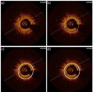
However, even though the existing techniques show good results, there is still a need of a robust and eficient method to obtain the stent area from coronary arteries FD-IOCT images. For that reason, the present paper focused on developing a method that segments the area contained by stent struts from FD-IOCT of coronary arteries (Figure 1), positioned either internally to the lumen or covered by plaque using two different strategies (Moving Window Iterative Ellipses and Cylinder Fitting). A part of these strategies was presented on the VII Instrumentation and Medical Image Symposium in Campinas – Brazil (Gaiarsa et al., 2015).
Methods
The FD-OCT equipment (C7-XR, St. Jude Medical) was used to obtain the images, having nominal pullback speed of 20mm/sec. For the development of the method, three FD-IOCT image sequences were used, corresponding
to 443 2D images provided by the Heart Institute (InCor) with their respective ethics committee approval (number SDC 2929/07/004).
The method was divided into three steps: pre-processing, processing and post-processing. In the pre-processing step, the focus was to highlight important features removing unwanted objects; in the processing step, techniques were developed to ind possible stent strut candidates; whereas in the post-processing step two strategies were created to ind the best ellipse contained by the already found candidates.
Pre-processing
Initially, the images acquired in DICOM format were manually selected, removing the beginning and ending of the sequence to contain only the stented coronary images.
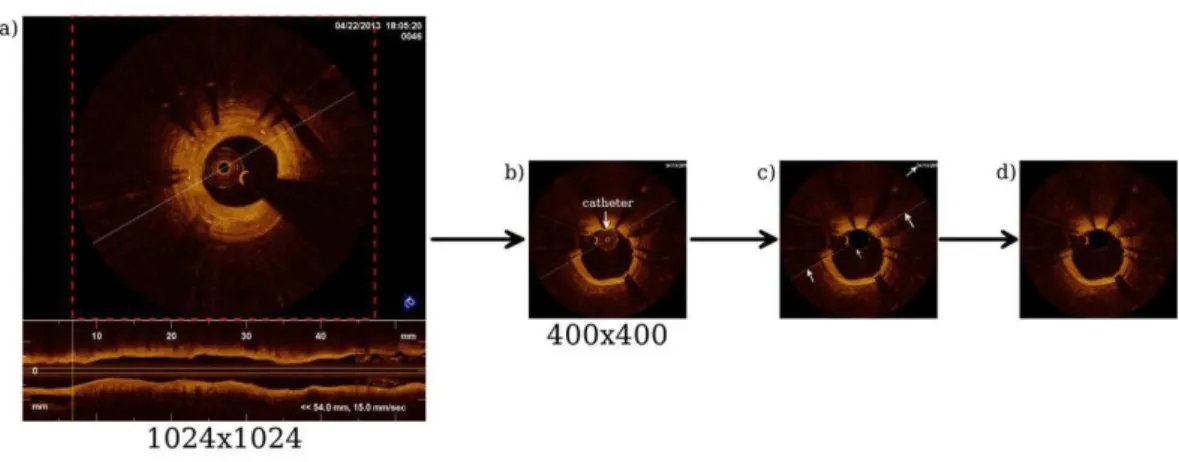
For every slice (2D image) a size normalization to 400x400 pixels was performed (Figure 2a) to later remove unwanted objects. One of the unwanted objects is the catheter relex (or catheter), which is a round structure generated by the relex of the light on the catheter (Figure 2b). It was identiied and removed based on its location (centered), format (round) and size (radius of 26 pixels).
In addition, there are some characteristics that are automatically inserted in the image by the equipment, and were removed by the recognition of the color yellow or white as seen in Figure 2c.
Figure 1. Example of (a) a slice, (b) stent area segmented manually, (c) stent area segmented by the ellipse itting method and (d) stent area
Processing
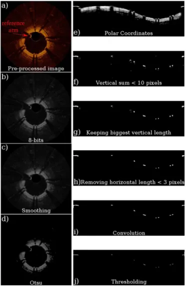
In this step we segmented the stent struts in different locations. Initially, two consecutive procedures were executed on all images, the irst segmented stent struts positioned inside the lumen and the second segmented the ones covered by plaque. Later, the relection of the reference arm (Figure 3a) was located and removed, preventing it from being mistaken for a stent strut since it has very similar characteristics.
Stent positioned inside lumen
For this procedure, irst the images were transformed into gray levels (8 bits) (Figure 3b), and then they were smoothed with a 3x3 neighborhood mean ilter (Figure 3c). After that, an Otsu threshold (Otsu, 1979) was found, maintaining pixel’s intensity when above the threshold, removing the other ones (changing their intensity to zero) (Figure 3d). Also, Cartesian Coordinates were converted to Polar Coordinates (Figure 3e), and each vertical line was iltered removing regions with length bigger than 10 pixels (Figure 3f) – considered as vessel wall – isolating possible stent candidates. To eliminate noise, vertical lines (A-lines) were again analyzed, keeping in each line the region with the greatest sum of connected pixels with intensity value bigger than zero (Figure 3g). And to eliminate remaining pieces of the lumen wall, horizontal lines were analyzed, removing connected regions smaller than 3 pixels (Figure 3h). To reveal regions with an abrupt increase and decrease of intensity – a stent strut characteristic – a derivative convolution (Equation 1) was applied (Figure 3i), and then the images were transformed to binary with a threshold of 170 (chosen empirically), highlighting the stent candidates (Figure 3j).
( ) ( )
1 1 1
, 0 0 0 * ,
1 1 1
− − −
θ = θ
conv conv
I r I r (1)
where Iconv
( )
θ,r is the image after the convolution and( )
θ,nconv
I r is the image before the convolution.
Stent covered by plaque
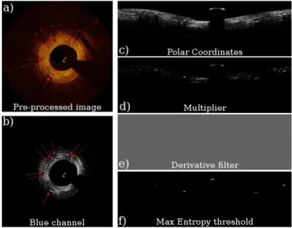
To isolate stent struts covered by plaque we conducted contrast tests on intensity proiles from different color channels (RGB) and found that the color that most highlights the plaque covered stents is the blue one. Therefore, in this procedure the images were converted to 8 bits from the pre-processing step using only the blue channel (Figure 4b). After that, they were transformed to Polar Coordinates (Figure 4c), and to emphasize the intensity peaks, irst each pixel’s intensity was raised to the 4th power (Figure 4d) to then apply the derivative ilter (Figure 4e) from Equation 2.
( )
θ, =2( )
θ, −(
θ + −, 2)
(
θ −, 2)
D P P P
I r I r I r I r (2)
where IP is the image before the ilter and ID after. To isolate possible candidates a MaxEntropy thresholder (Kapur et al., 1985) was used (Figure 4f).
Identifying the reference arm
To select the stented area properly it is important to merge the “covered” with the “inside lumen” candidates’ images and then remove the relection of the reference arm from them. The irst steps used in this process were the same from Figure 2, but without the “keeping biggest vertical length” step (“g” step) and using a binary threshold of 50 (chosen empirically) in the thresholding step (“j” step), removing most non-reference-arm pixels. After that, the reference arm region was located through
Figure 2. Pre-processing sequence: (a) Original 2D image; (b) Normalized into 400x400 pixels and with identiication of the catheter; (c) Catheter
the identiication of the biggest horizontal connection (Figure 5).
Finally, after isolating the candidates, the images were transformed back to Cartesian Coordinates.
Post-processing
In the post-processing step, the stented area was selected. Although there are good results in segmenting stent struts found in the literature, this study was focused in inding the areas comprised by stent even with false positives and false negatives detection of stent struts. With that in mind, two strategies were developed, compared and evaluated.
Moving Window Iterative Ellipses
In the irst strategy, we called “Moving Window Iterative Ellipses” (MWIE), the area contained by stent struts was considered elliptical.
Due to the fact that the stent struts’ position doesn’t change abruptly in consecutive slices, it was possible to use in each slice stent information from its neighborhood in a moving window fashion. That is, each slice was updated to the result of an OR operation between the binary information contained in itself and n neighbor slices from each side. This procedure was used because of the dificulty of obtaining enough information from every slice, providing more points and more conidence for the outlining of ellipses.
To ind the ellipse in each slice (after the joining of stent information from neighbor slices) the following ellipse itting method based on Halir and Flusser (1998) was used.
An ellipse is a special case of a conic section and can be represented by the following polynomial:
( ) 2 2
, = + + + + + =0
F x y ax bxy cy dx ey f (3)
with an ellipse-speciic constraint
2
4ac−b =1 (4)
Taking into account the following vectors:
[ , , , , , ]
= T
A a b c d e f (5)
2, , 2, , ,1
=
X x xy y x y (6)
and rewriting the Equation 3 as
( )
= ⋅ =0A
F X X A (7)
the minimization of the algebraic distance from the points
(
x yi, i)
can be calculated as:( )
(
)
2(
( ))
21 1
,
= = =
∑N ∑N
A A i i A A i
i i
min F x y min F X (8)
( )2
1
= ⋅
= A∑N i
i
min X A
From this algorithm, in each slice an ellipse was automatically outlined using as input parameters (to the Halir and Flusser (1998) method) the stent strut candidates yielded (Equation 8) in the processing step. Next, an iterative process took place, where in each iteration the pixels farthest from the ellipse were removed and Figure 4. Steps used in segmenting stent struts in covered position.
a new ellipse was drawn based on the remaining stent strut candidates until the maximum distance between the ellipse and the struts was 5 pixels.
The iterative process increases the probability of inding a closer-to-real area, even with the existence of false positive candidates.
Cylinder itting
In this second strategy (CF), following a proposal that the stent is a cylindric structure, a method was developed minimizing the distances between the points (stent strut candidates) and cylinders.
Assuming that there was an angle between the catheter and the artery, the ellipses would also have a slope in relation to the cylinder. Using this approach, an iterative process was created minimizing the distance between points to cylinders in a moving 3D window.
a. Finding the axis of the cylinder
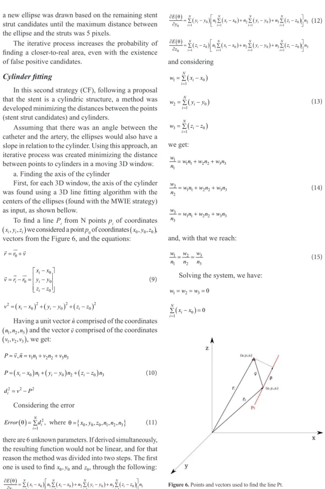
First, for each 3D window, the axis of the cylinder was found using a 3D line itting algorithm with the centers of the ellipses (found with the MWIE strategy) as input, as shown bellow.
To ind a line Pt from N points pi of coordinates
(
x y zi, i, i)
we considered a point p0 of coordinates(
x y z0, 0, 0)
, vectors from the Figure 6, and the equations:0
= +
r r v
0 0 0 0 − = − = − − i i i i x x
v r r y y
z z
(9)
( ) (2 ) (2 )2
2
0 0 0
= i− + i− + i−
v x x y y z z
Having a unit vector nˆ comprised of the coordinates
(
n n n1, 2, 3)
and the vector v comprised of the coordinates(
v v v1, 2, 3)
, we get:1 1 2 2 3 3
,
= = + +
P v n v n v n v n
(
0)
1(
0)
2(
0)
3= i− + i− + i−
P x x n y y n z z n (10)
2= 2− 2
i
d v P
Considering the error
( ) 2
1 , = θ = ∑N i
i
Error d where θ =
{
x y z n n n0, 0, 0, ,1 2, 3}
(11)there are 6 unknown parameters. If derived simultaneously, the resulting function would not be linear, and for that reason the method was divided into two steps. The irst one is used to ind x y0, 0 and z0, through the following:
( ) ( ) ( ) ( ) ( )
0 1 0 2 0 3 0 1
1 1 1 1
0 = = = =
∂ θ =∑ − ∑ − + ∑ − + ∑ −
∂
N N N N
i i i i
i i i i
E
x x n x x n y y n z z n
x
( ) ( ) ( ) ( ) ( )
0 1 0 2 0 3 0 2
1 1 1 1
0 = = = =
∂ θ =∑ − ∑ − + ∑ − + ∑ −
∂
N N N N
i i i i
i i i i
E
y y n x x n y y n z z n
y (12)
( ) ( ) ( ) ( ) ( )
0 1 0 2 0 3 0 3
1 1 1 1
0 = = = =
∂ θ =∑ − ∑ − + ∑ − + ∑ −
∂
N N N N
i i i i
i i i i
E
z z n x x n y y n z z n
z and considering ( ) 1 0 1 = =∑N i−
i
w x x
( )
2 0
1 = =∑N i−
i
w y y (13)
( )
3 0
1 = =∑N i−
i
w z z
we get:
1
1 1 2 2 3 3
1
= + +
w
w n w n w n n
2
1 1 2 2 3 3
2
= + +
w
w n w n w n
n (14)
3
1 1 2 2 3 3
3
= + +
w
w n w n w n n
and, with that we reach:
3
1 2
1 2 3
= =w
w w
n n n (15)
Solving the system, we have:
1= 2= 3=0
w w w
( 0)
1
0
= − =
∑N i i
x x
( 0) 1
0
= − =
∑N i i
y y (16)
( 0)
1
0
= − =
∑N i i
z z
And inally, isolating x y0, 0 and z0 we get:
1
0 =
∑ = iNxi x N 1 0 = ∑ = Ni yi y N (17) 1 0 = ∑ = iNzi z
N
showing the possibility to ind x y0, 0 and z0without knowing n n1, 2 and n3.
In the second step, to ind n n1, 2 and n3, Lagrange Multipliers were used with the same Error from Equation 11 and the following constraint:
2 2 2
1 + 2+ 3=1
n n n therefore
(
2 2 2)
1 2 3 1 0
λ n +n +n − = (18)
coming up with
( )
{
2 ( ) ( ) ( ) 2}
2 2 21 0 0 1 0 2 0 3 1 2 3
1
, ( 1)
=
λ =∑ − − − + − + − + λ + + −
N
i i i
i
L n r r x x n y y n z z n n n n (19)
Deriving the Equation 19 of function of n n1, 2 and n3 and equaling to zero we have:
( )2 ( )( ) ( )( )
1 0 2 0 0 3 0 0 1
1 1 1
1
0
= = =
∂ = ∑ − + ∑ − − + ∑ − − − λ =
∂
N N N
i i i i i
i i i
L
n x x n y y x x n z z x x n
n
( )( ) ( )2 ( )( )
1 0 0 2 0 3 0 0 2
1 1 1
2
0
= = =
∂ = − − + − + − − − λ =
∑ ∑ ∑
∂
N N N
i i i i i
i i i
L
n x x y y n y y n z z y y n
n (20)
( )( ) ( )( ) ( )2
1 0 0 2 0 0 3 0 3
1 1 1
3
0
= = =
∂ = − − + − − + − − λ =
∑ ∑ ∑
∂
N N N
i i i i i
i i i
L
n x x z z n y y z z n z z n
n
And, therefore
( )2 ( )( ) ( )( )
1 1 1
1∑= − 0 + 2∑= − 0 − 0 + 3∑= − 0 − 0 =λ1
N N N
i i i i i i i i
n x x n y y x x n z z x x n
N N N N
( )( ) ( )2 ( )( )
1 1 1
1∑iN= i− 0 i− 0 + 2∑iN= i− 0 + 3∑iN= i− 0 i− 0 =λ2
n x x y y n y y n z z y y n
N N N N (21)
( )( ) ( )( ) ( )2
1 1 1
1∑= − 0 − 0 + 2∑= − 0 − 0 + 3∑= −0 =λ3
N N N
i i i i i i i i
n x x z z n y y z z n z z n
N N N N
transforming into:
2 1
1 2 3
λ σ + σ + σ =x xy xz n
n n n
N
2 2
1 2 3
λ σ + σ + σ =xy y yz n
n n n
N (22)
2 3
1 2 3
λ σ + σ + σ =xz yz z n
n n n
N And 2 1 1 2 2 2
2 3 3
σ σ σ
λ
σ σ σ ⋅ =
σ σ σ
x xy xz
xy y yz
xz yz z
n n n n N n n (23) translating into:
⋅ = λ
A n n (24)
Finally, representing the greatest variance, the optimal eigenvalue is the biggest with its corresponding eigenvector.
b. Finding the cylinder radius
After the axis was found, the following process to minimize the distances between the points and cylinders was created.
Assuming a point Pt, its distance to the cylinder dc is
= −
c i
d d R, where di is the distance from Pi to the cylinder axis and R is the cylinder radius. For the minimization, the following error was considered:
( ) ( )2
1 = =∑N i−
i
Error R d R (25)
and minimized as:
( ) ( )( )
1
2 1 0
= ∂ =∑ − − = ∂ N i i Error R d R R 1 1 . = = = = ∑N i ∑N
i i
d R N R (26)
1 =
∑ = iNdi R
N
c. Finding the distances between points and cylinder To ind di we suppose a vector 0
P A with a projection
0
P B on a line Pt with equation Pt=P0+tv. Therefore:
( )
0 = 0
v
P B Proj P A
0 0 2 = ⋅
P A v
P B v
v (27) with 0 0 = −
BA P A P B
2 2 2
0 0
= −
BA P A P B (28)
replacing (27) in (28):
(
)
22 0 0 2 = − ⋅
P A v BA P A
v
d. Removing unwanted points
After being able to calculate the distances between the cylinder and the points, in each iteration the farthest points were removed and a new cylinder was found. That process was done until the maximum distance calculated was 20% of the cylinder radius.
Results
To reach the main goal of segmenting the area contained by stent struts, two strategies were developed and tested. The results compare the area found through the methods with the area found manually by specialists.
Both strategies used the same pre-processing and processing steps, and therefore they used also the same points for stent strut candidates. They were applied to 3 different DICOM sequences with different characteristics. The irst one has 93 slices, the second 182 and the third 168, totaling 443 slices. The results are also presented according to the speciic sequence and totalized.
All the algorithms were developed and executed through ImageJ plugins in Java on a personal Dell computer with Intel Core 2 Duo 2.93 GHz processor, 4 GB of RAM and Linux Mint 16 Cinnamon 64-bits operational system.
Two evaluation metrics were used comparing the stented area found by our methods with the stented area found manually. In the irst one, proposed by Udupa et al. (2006), the mean and standard deviation were calculated for true positives and false positives. The second one, called Hausdorff Metric (Huttenlocher et al., 1993), measures how far two contours are from each other.
For a better understanding of the resulting values, the Hausdorff distance is presented as a percentage of the mean lumen diameter (measured manually).
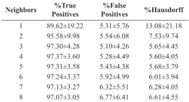
Evaluating moving window iterative ellipses The irst step in the ellipse itting algorithm is to join a certain number of neighbor slices in a moving window fashion. With the purpose of inding the optimal value for slice neighbor quantity values from 1 to 8 were tested. As displayed on Table 1, the best quantity of neighbors is between 3 and 5, wherein 4 was considered the optimal value. The obtained data show that in spite of the different characteristics from the sequences the results stay stable, accurate and precise.
The run time of this strategy highly depends on the chosen parameters. The neighbor’s quantity is the most signiicant one, and it mainly affects the iterative part of the algorithm because the more neighbors are chosen, the more points are present and the more iterations have to be executed. We veriied that the execution time of the algorithm with 4 neighbors was close to 0.51 seconds per slice (0.30 seconds of pre-processing and
processing + 0.21 seconds of iterative process) and that the time consumed by the iterative part is approximately proportional to the number of neighbors.
Evaluating cylinder itting
Arranging tested data as the previous item, Table 2 shows the totalized results. The parameters tested were neighbor quantity (3 to 5 slices) and cylinder length (5, 10, 15 and 20 slices).
Although there are not signiicant differences between parameters, the best results are shown with 4 neighbors and cylinder size 10. In addition, in comparison to the results from the MWIE strategy the present shows little improvement, being virtually equivalent.
In this strategy, the run time becomes greater because in each cylinder iteration the ellipse iterations are also executed. Therefore, it should be considered that the MWIE is executed many times until a proper cylinder is found. The execution time also depends on the set of parameters, increasing signiicantly with the cylinder size. On average, for a size 10 cylinder the run time was 55,67 seconds per slice and for a size 5 cylinder the run time was 25,51 seconds per slice.
Discussion
To monitor CHD patients and avoid waste of specialists’ time, the objective of this study was the development of a method that segments the area contained by stent struts from FD-IOCT of coronary arteries. To achieve this purpose two strategies were created and tested.
Unlike previous studies, that focus on segmenting objects (stent struts), the present work segments an area, presenting useful results to the medical ield.
Two strategies were proposed and developed to segment the area contained by stent struts. In the Moving Window Iterative Ellipses (MWIE), 2D slice information was used relating neighbors to outline ellipses, while in the Cylinder Fitting (CF), it was proposed that the points found were positioned along a cylinder wall. The results show that there are not signiicant accuracy
Table 1. Results of the strategy “Moving window iterative ellipses” totalized (443 slices).
Neighbors %True
Positives
%False
Positives %Hausdorff
differences between the two strategies tested while the CF execution time is at least 50 times greater than the MWIE. Therefore, because the MWIE and CF results were so similar, it is reasonable to say that the MWIE strategy can also be considered as a simpler and faster approximation of the CF algorithm.
The main contributions of this projects are: irst, the usage of the information contained in neighbor slices, providing more conidence in locating stent struts; second, considering the stent area region an ellipse, allowing an optimization approach; third, outlining ellipses in a iterative process, removing unnecessary information and making the area closer to real; and fourth, simulating that the stent longitudinal portion has a cylindric shape, obtaining results that prove the accuracy of the method.
However, some limitations must be noted. The manual segmentation, considered as the gold standard, is a critical factor in the medical image area. There are problems such as incoherence in determining boundaries and increasing error due to fatigue. In addition, this study was created for FD-IOCT images, and restricted to the provided images (3 DICOM sequences). The distance between two consecutive slices was approximated to 200µm due to the equipment’s nominal pullback speed (20 mm/s) and frame rate (100 fps). With this coniguration, we estimated the optimal number of neighbors to be 4. This number may differ depending on the equipment and settings used for the image acquisition, which should be brought to attention when trying to reproduce the method. Although the sequences showed different characteristics, it would be ideal to test the method with a larger variety. Some speciic limitations of the method include the relatively long processing time needed for the CF strategy and the use of ixed thresholds when segmenting stent struts. Nevertheless, the use of ixed thresholds was proven necessary through a study comparing the MWIE strategy with 4 neighbors, obtaining results for the method without ixed thresholds of total True Positives of 94.17 ± 6.74, total False
Positives of 4.30 ± 7.96 and total Hausdorff distance of 7.79 ± 9.52; in comparison with the method with ixed thresholds of total True Positives of 97.37 ± 3.60, total False Positives of 5.28 ± 4.49 and total Hausdorff distance of 5.60 ± 4.05. Therefore, we conclude that the ixed thresholds improve the results when the images show regions with lower wall intensity, generating false positives that are removed by the thresholds.
Therefore, a larger image database is desirable for future work. Further investigation would be the geometric reconstruction of the coronary artery based only on the images and the FC strategy, which can estimate the location of the catheter with respect to the stent.
Acknowledgements
We thank the Heart Institute (InCor) for providing the images; Brazil’s National Council of Technological and Scientiic Development (CNPQ) for the inancial support; and 2 anonymous reviewers for their comments and suggestions.
References
Bezdek JC, Ehrlich R, Full W. FCM: the fuzzy c-means clustering algorithm. Computers & Geosciences. 1984; 10(2):191-203. http://dx.doi.org/10.1016/0098-3004(84)90020-7.
Bezerra HG, Costa M, Guagliumi G, Rollins AM, Simon DI. Intracoronary optical coherence tomography: a comprehensive review clinical and research applications. JACC: Cardiovascular Interventions. 2009; 2(11):1035-46. PMid:19926041. http:// dx.doi.org/10.1016/j.jcin.2009.06.019.
Cohen B, Hasselbring B. Coronary heart disease: a guide to diagnosis and treatment. 2nd ed. Omaha, Nebraska: Addicus Books; 2007.
Gaiarsa V, Cardenas D, Furuie S. Seleção semi-automática de área contida por stent em FD-IOCT utilizando imagens sequenciais. In: Anais do 7° Simpósio de Instrumentação e Imagens Médicas; 6° Simpósio de Processamento de Sinais da
Table 2. Results of the strategy “Cylinder itting” totalized (443 slices).
Neighbors Cylinder size %True Positives %False Positives %Hausdorff
3 5 97.37±3.03 4.88±4.08 4.83±3.55
3 10 97.52±2.25 4.55±3.32 4.46±1.99
3 15 97.38±2.30 5.09±3.47 4.87±2.11
3 20 97.12±2.48 5.08±3.76 5.07±2.42
4 5 97.53±2.27 5.03±4.15 4.78±3.03
4 10 97.52±2.26 4.68±3.46 4.53±2.06
4 15 97.42±2.33 5.12±3.57 4.86±2.14
4 20 97.12±2.53 5.13±3.82 5.06±2.42
5 5 97.49±2.37 5.17±4.04 4.82±2.47
5 10 97.47±2.35 4.87±3.78 4.66±2.20
5 15 97.40±2.40 5.22±3.74 4.92±2.23
UNICAMP. 2015 Out 21-23; Campinas, São Paulo. Campinas: Editora Atual; 2015. p. 129-132.
Halir R, Flusser J. Numerically stable direct least squares fitting of ellipses. In: Proceedings of the 6th International Conference in Central Europe on Computer Graphics and Visualization. 1998 Feb 9-13; Plzen, Czech Republic. Plzen: Vaclav Skala Union Agency; 1998. v. 98. p. 125-32.
Huttenlocher DP, Klanderman G, Rucklidge WJ. Comparing images using the Hausdorff distance. IEEE Transactions on Pattern Analysis and Machine Intelligence. 1993; 15(9):850-63. http://dx.doi.org/10.1109/34.232073.
Kapur JN, Sahoo PK, Wong AKC. A new method for gray-level picture thresholding using the entropy of the histogram. Computer Vision Graphics and Image Processing. 1985; 29(3):273-85. http://dx.doi.org/10.1016/0734-189X(85)90125-2.
Li SZ. Markov random field modeling in computer vision. Singapore: Springer Science & Business Media; 1995.
Mallat S, Hwang WL. Singularity detection and processing with wavelets. IEEE Transactions on Information Theory. 1992; 38(2):617-43. http://dx.doi.org/10.1109/18.119727.
Mandelias K, Tsantis S, Spiliopoulos S, Katsakiori PF, Karnabatidis D, Nikiforidis GC, Kagadis GC. Automatic quantitative analysis of in-stent restenosis using FD-OCT in vivo intra-arterial imaging. Medical Physics. 2013; 40(6):63101. PMid:23718609. http://dx.doi.org/10.1118/1.4803461.
Mittal S. Coronary heart disease in clinical practice. London: Springer Science & Business Media; 2005.
Otsu N. A threshold selection method from gray-level histograms. IEEE Transactions on Systems, Man, and Cybernetics. 1979; 9(1):62-6. http://dx.doi.org/10.1109/TSMC.1979.4310076.
Tsantis S, Kagadis GC, Katsanos K, Karnabatidis D, Bourantas G, Nikiforidis GC. Automatic vessel lumen segmentation and stent strut detection in intravascular optical coherence tomography. Medical Physics. 2012; 39(1):503-13. PMid:22225321. http:// dx.doi.org/10.1118/1.3673067.
Udupa JK, LeBlanc VR, Zhuge Y, Imielinska C, Schmidt H, Currie LM, Hirsch BE, Woodburn J. A framework for evaluating image segmentation algorithms. Computerized Medical Imaging and Graphics. 2006; 30(2):75-87. PMid:16584976. http:// dx.doi.org/10.1016/j.compmedimag.2005.12.001.
Ughi GJ, Adriaenssens T, Onsea K, Kayaert P, Dubois C, Sinnaeve P, Coosemans M, Desmet W, D’hooge J. Automatic segmentation of in-vivo intra-coronary optical coherence tomography images to assess stent strut apposition and coverage. International Journal of Cardiac Imaging. 2012; 28(2):229-41. PMid:21347593. http://dx.doi.org/10.1007/s10554-011-9824-3.
Wang A, Eggermont J, Dekker N, Garcia-Garcia HM, Pawar R, Reiber JH, Dijkstra J. Automatic stent strut detection in intravascular optical coherence tomographic pullback runs. International Journal of Cardiac Imaging. 2013; 29(1):29-38. PMid:22618433. http://dx.doi.org/10.1007/s10554-012-0064-y.
Wang Z, Jenkins MW, Linderman GC, Bezerra HG, Fujino Y, Costa MA, Wilson D, Rollins A. 3-D stent detection in intravascular OCT using a Bayesian network and graph search. IEEE Transactions on Medical Imaging. 2015; 34(7):1549-61. PMid:25751863. http://dx.doi.org/10.1109/TMI.2015.2405341.