A HEURISTIC FOR THE
MINIMIZATION OF OPEN STACKS PROBLEM
Fernando Masanori Ashikaga*
FATEC São José dos Campos Centro Paula Souza
São José dos Campos – SP, Brazil [email protected]
Nei Yoshihiro Soma
Computer Science Division
Technological Institute of Aeronautics São José dos Campos – SP, Brazil
* Corresponding author / autor para quem as correspondências devem ser encaminhadas
Recebido em 05/2008; aceito em 04/2009 após 1 revisão Received May 2008; accepted April 2009 after one revision
Abstract
It is suggested here a fast and easy to implement heuristic for the minimization of open stacks problem (MOSP). The problem is modeled as a traversing problem in a graph (Gmosp) with a special structure
(Yanasse, 1997b). It was observed in Ashikaga (2001) that, in the mean experimental case, Gmosp has
large cliques and high edge density. This information was used to implement a heuristic based on the extension-rotation algorithm of Pósa (1976) for approximation of Hamiltonian Circuits. Additionally, an initial path for Pósa’s algorithm is derived from the vertices of an ideally maximum clique in order to accelerate the process. Extensive computational tests show that the resulting simple approach dominates in time and mean error the fast actually know Yuen (1991 and 1995) heuristic to the problem.
Keywords: minimization of open stacks; extension-rotation heuristic; clique.
Resumo
Sugerimos uma heurística rápida e de implementação simples para o problema de minimização de pilhas abertas (MOSP). O problema é modelado como um problema de percorrimento de arcos no grafo (Gmosp) associado (Yanasse, 1997b). Foi observado em Ashikaga (2001) que o grafo Gmosp possui
grandes cliques e uma alta densidade de arestas. Esta informação foi utilizada para implementar uma heurística baseada no algoritmo Extensão-Rotação de Pósa (1976) para aproximação de Circuitos Hamiltonianos. O caminho inicial para o algoritmo de Pósa é obtido a partir dos vértices de uma aproximação do maior clique do grafo para acelerar o processo. Testes computacionais extensivos mostram que a abordagem domina tanto em tempo quanto em erro médio a mais rápida heurística conhecida de Yuen (1991 e 1995).
1. Introduction
The Minimization of Open Stacks Problem (MOSP) is defined by a set of piecesΠ = {1,… n} and a set Λ = {P1,… Pm} of patterns, each Pj, j = 1,…, m, is formed by a non-empty subset of pieces from Π. Any piece ρ
∈
Π
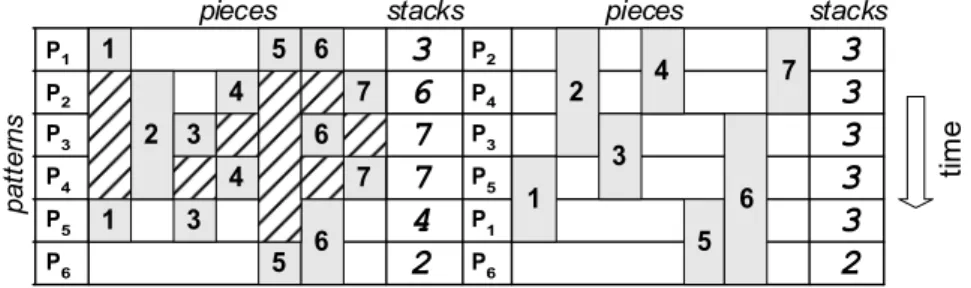
is processed by a single machine (M) and it remains around M in an openstack of pieces of the same ρ typeuntil its demand is fulfilled, the stack is considered closed when all patterns Pj containing the piece ρ are cut. The objective of the problem is to schedule the order in which M will process the patterns such that the maximum number of open stacks is minimized. The MOSP appears, e.g., in the context of wood cutting where there is a limited storage space around a saw machine and stacks of panels being cut have to be removed only after their orders are completed. Figure 1 presents a small example of two sequences of patterns (Spa’s) with the corresponding stacks opened during the cutting process. For Spa = {1, 2, 3, 4, 5, 6}, seven stacks are opened, while for Spa = {2, 4, 3, 5, 1, 6} just three stacks are used during the entire process. A shaded area indicates that a stack associated to a given piece remains open while its demand is not fulfilled. For instance, a stack containing piece 4 remains open while patterns P2, P3 and P4 are processed, cf. left side of Figure 1.1 1 2 3 3 4 4 5 5 6 6 6 7 7 1 2 3 4 5 6 7 P1 P2 P3 P4 P5 P6 P2 P4 P3 P5 P1 P6
3
6
7
7
4
2
3
3
3
3
3
2
stacks stacks pieces pieces p a tte rn s ti m eFigure 1 – Open stacks for Spa = {1,2,3,4,5,6} and Spa = {2,4,3,5,1,6}.
The MOSP models a variety of industrial situations, such as VLSI design (Ferreira & Song, 1992), wood and glass cutting (Yanasse, 1997a; Yuen, 1991 and 1995). Additionally, the problem is also known to be NP-Hard (Linhares & Yanasse, 2002) and therefore, difficult to be solved exactly. In Becceneri et al. (2004) it is presented the best heuristic, up to now, in terms of the quantity of open stacks, despite a much worst running time than Yuen (1995) and our new heuristic presented here. Metaheuristics solutions for the MOSP were also suggested (Faggioli & Bentivoglio, 1998; Fink & Voss, 1999).
sections are organized as follows: in Section 2 we present the major idea of the well known Yuen (1995) algorithm for MOSP, in Section 3 the algorithm suggested here is given in details. In Section 4 the computational experiments are presented and the conclusions are given in Section 5.
2. The Yuen heuristic
In Yuen (1995) five heuristics for solving the MOSP are suggested and the third one, Yuen3, is considered as the best one so far to the problem in terms of the tradeoff between computational time and mean error (Yuen, 1995; Becceneri, 1999). The idea behind Yuen3 is to select a pattern that shares the largest number of common pieces with the current open stacks and it is based on the following three metrics: Cj is the number of piece types common to pattern j and the current open stacks; Nj is the number of different pieces in pattern j not included in the current open stacks and Mj is defined as the number of piece types common to pattern j and the current open stacks less the number of new piece types or potential stacks contained in that pattern. This difference, Mj = Cj - Nj tries to appraise the impact that a given choice of pattern j to be cut has in relation with the pieces contained in it. Therefore, this local information is used as a guide to the search of smaller quantities of different new stacks. The criterion to select a pattern to be sequenced is dictated by non-increasing values of Mj. A tie is broken in favor of a pattern with the lowest Nj value and if it still persists the one with lowest index j is chosen. This heuristic has a straightforward implementation and its running time is bounded by O(n3).
3. The new Ashikaga Soma (AS) heuristic
The graph model for the MOSP used here was introduced in Yanasse (1997a) and the idea is to associate a vertex to a piece and a clique to a pattern, an edge represents two pieces present in a same pattern. Moreover, parallel arcs are counted and represented as a single one. In Ashikaga (2001) it was shown that, in general, a MOSP graph has very large maximum cliques in comparison with those randomly generated ones; i.e. it has large deviations from expected clique values (Bollobás, 2001).
The new traversing problem in this MOSP graph is presented in Yanasse (1997b), “follow the sequence of the arcs and sequence a pattern Pj when, for the first time, all the vertices corresponding to all the pieces types in Pj are open”. An arc indicates that the corresponding vertices associated with pieces belong to at least a pattern Pj. By sequencing all the vertices of the graph that are connected via arcs corresponds to a general and broad policy. The sequence of arcs in this traversing problem is also used by the present suggested approach.
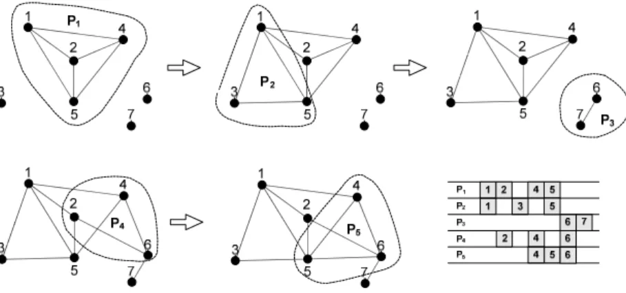
Figure 2 shows how a MOSP graph is generated from a matrix of patterns, e.g., pattern P5 has 4 types of pieces: 3, 6, 7 and 10.
8
9
4 3
1 5
10
7
6
2
4 4
8 6
6
6 7
7
3 5
7 1
2
9 P1
P2
P3
P4
P5
P6
P9
P8
P7
P10
3 1
1
1 2
3
3 5
9 10
10
10
P 5
Figure 2 – MOSP graph with corresponding matrix of patterns.
Figure 3 – The process of construction of Gmosp by a union of clique patterns.
It is well known that finding a maximum clique is NP-Hard (Garey & Johnson, 1979). However, for dense graphs, as it is the case for the MOSP, in the mean experimental case, greedy algorithms for finding a clique cannot generate bad results (Homer & Peinado, 1996; Kučera, 1995).
A graph is complete, denoted by Kn, if all of their n vertices are mutually adjacent. A clique is a subset of Kn. A complement graph G’ of G is such that the vertices are the same in both graphs and an edge belongs to G’ if and only if it is not present in G. A clique number of a graph G, denoted by ω(G), is the maximal number of vertices of a clique in G (Bollobás, 1998).
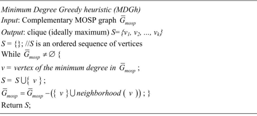
The independent set problem is that of finding a mutually non-adjacent vertices set of a graph. A clique is its dual problem and it consists of detecting a set of adjacent vertices. Therefore, if S is a maximal independent set in a given graph it also is a maximal clique in its complement graph. In order to obtain an approximation of maximum clique we used the complement graph and the Minimum Degree Greedy heuristic for independent sets, which performs well in sparse graphs (original complement graphs are dense), cf. Halldórsson & Radhakrishnan (1994).
Minimum Degree Greedy heuristic (MDGh) Input: Complementary MOSP graph Gmosp
Output: clique (ideally maximum) S={v1, v2, ..., vk} S = {}; //S is an ordered sequence of vertices While Gmosp≠ ∅{
v = vertex of the minimum degree in Gmosp;
S = S∪
{ }
v ;{ }
( )
(
)
mosp mosp
G =G − v ∪neighborhood v ; } Return S;
For the example of Figure 2, a maximum clique is obtained and S= {6,7,3,2,1}. Recall that a vertex in S corresponds to a piece to be cut by the saw machine and since S is an ordered set, the order in which the pieces have to be cut is dictated also by S. Moreover, from that set it is immediate to determine the sequence of patterns (Spa) to be processed and in a time bounded by O(n2). Figure 4 illustrates the process of MDGh in MOSP graph of Figure 3.
Figure 4 – MDGh heuristic.
Extension Rotation heuristic (Erh)
Input: MOSP Graph Gmospand S generated by the MDGh. Output: Extended S, via a Hamiltonian path.
Initialize xk and j properly; while (xk ≠∅ or j≠∅) {
xk = ´max degree neighbor of last vertex in S´; if xk ≠∅
S = S ∪xk; else {
j =´ some neighbor of the last vertex in the current path´; if j≠∅
create_another_path_with_the_same_vertex_set;
// revert the orientation of the subpath between j and last vertex }
} Return S;
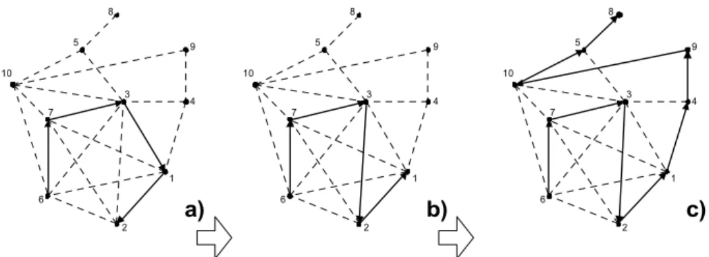
Figure 5 shows that MDGh returns an initial S = {6, 7, 3, 1, 2}. An initial path given by vertices 6-7-3-1-2 has no further vertex to extend (Figure 5a). Since there is an arc between vertices 3 and 2, a rotation follows, modifying thus the path to 6-7-3-2-1 (Figure 5b). After that it is possible to further perform 5 more extensions (Figure 5c) and S = {6, 7, 3, 2, 1, 4, 9, 10, 5, 8}, the given solution is optimal to this example.
8
9
4 3
1 5
10
7
6
2
8
9
4 3
1 5
10
7
6
2
8
9
4 3
1 5
10
7
6
2
a) b) c)
Figure 5 – Extension-Rotation Heuristic.
8
9
4 3
1 5
10
7
6
2
4 4
8 6
6
6 7 3
5 7 1
2
9 p9
p10 p3 p2 p8 p
4
p
1
p
5
p
7
p6
3
S={6, 7, 3, 2, 1, 4, 9, 10, 5, 8} Spa={9, 10, 3, 2, 8, 4, 7, 5, 1, 6}
2
1
7 1
1 3
9 10 10
3 10
5
Figure 6 – S and the corresponding sequence of patterns (Spa).
An experimental determined limit of two rotations was imposed to Erh. This constraint implies that, in principle, not all vertices (pieces) will be traversed (sequenced) since a Hamiltonian path may not be found. For the eventuality of existence of vertices yet to be sequenced some of them can be neighbors to the ones generated after MDGh and Erh. To this case such a vertex is called a conjugated and the others as remaining. At this point set Π is partitioned into three subsets: Π = S∪Conj∪Rem, where S is given by the execution of MDGh and Erh, Conj by the conjugated and Rem by the remaining vertices. For ease of comprehension suppose that the example of Figure 2 has three additional vertices, C1, C2 and R as given in Figure 7. A solution for this problem given by MDGh and Erh and presented in Figures 5 and 6 implies that C1 and C2 belong to the set Conj while vertex R belongs to the set Rem.
Figure 7 – Conj and Rem Vertices in S = {7, 2, 6, 9, 4, 12, 10, 8, 11, 13, 1}.
the end of the sequence in a simple lexicographical manner. For the example given before, S becomes: S = {C2, 6, 7, 3, C1, 2, 1, 4, 9, 10, 5, 8, R}.
The following pseudo-code summarizes its major steps.
Ashikaga Soma (AS) Heuristic
Input: Set of pieces Π and set of patterns Λ; Output: Sequence of patterns (Spa) Generate Gmosp from Π and Λ; S := MDGh ( Kn - Gmosp ); S := Erh( Gmosp, S );
//Sequence remaining vertices
If there is any vertex yet to be sequenced
Detect and insert the conjugate vertices in S; Insert any left vertex in a lexicographical order in S; Generate Spa from S;
Return Spa;
Recall that Spa is obtained from S (ordered set) by traversing the set of vertices given by AS from the last to the first one, with the inclusion of the patterns that contains the vertex being considered. The worst-case complexity for the algorithm is O(n2), since MDGh is linear (Halldórson & Radhakrishnan, 1994). Each rotation can be made in O(log )n time (Angluin & Valiant, 1979), and the total number of extensions is at most O(n2) time. The conjugated and remaining vertices are inserted in S also in O(n2) time and the same to obtain the final sequence patterns generation. Hence, the total time is bounded by O(n2). As it will be presented next, the heuristic has a much better behavior in the practice than this theoretical worst case bound. Moreover, the heuristic has a speed up of a factor n in comparison with Yuen3, since this latter one is O(n3).
4. Computational Experiments
The suggested heuristic, AS, is compared with the Yuen3 algorithm. The first set of instances considered was suggested by Becceneri (1999) and covers the most common practical industrial scenario applications. In the second class a very large quantity of random instances were generated. The running times are expressed as CPU milliseconds in Table 1 and seconds in Table 2. The equipment is a Celeron 533 MHz with 64 Mbytes of main memory. All heuristics were implemented in Visual C++ 6.0.
For the tests it was assumed without loss of any generality that the quantity of pieces is equal to those of patterns since as observed by Yanasse (1997b) any pattern can either be grouped or divided into sets with exactly two pieces such that the total quantity of stacks remains the same in the optimal solution.
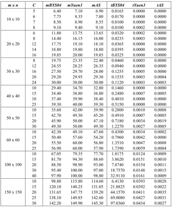
tBYS04, tYuen3 and tAS are the mean running time. For each case, the sample set has size 20 and it was randomly generated. It can be readily seen that BYS04 produces best results in terms of the quantity of open stacks, but at higher running times in relation to the number of patterns and pieces. Yuen3 and AS are very fast, but for increasing values of n, clearly, AS has a much better time performance than Yuen3. Also, AS produces a smaller quantity of open stacks than Yuen3 for larger values of n and is competitive with BYS04 for larger values of C.
Table 1 –Comparison of BYS04, Yuen3 and AS, (Becceneri et al., 2004) tests. Time expressed in milliseconds.
m x n C mBYS04 mYuen3 mAS tBYS04 tYuen3 tAS
5 6.40 7.10 6.90 0.0165 0.0000 0.0000 6 7.75 8.35 7.80 0.0170 0.0000 0.0000 7 8.50 8.90 8.55 0.0100 0.0000 0.0000 10 x 10
8 9.10 9.40 9.10 0.0100 0.0002 0.0000 6 11.80 13.75 13.65 0.0320 0.0002 0.0000 8 14.40 16.15 16.00 0.0235 0.0003 0.0000 12 17.75 19.10 18.10 0.0365 0.0000 0.0000 14 18.80 19.80 18.80 0.0395 0.0000 0.0000 20 x 20
16 19.85 20.00 19.85 0.0325 0.0000 0.0000 8 19.75 23.35 22.40 0.0460 0.0003 0.0000 12 24.55 28.25 26.35 0.0940 0.0000 0.0000 16 27.50 29.70 28.00 0.1255 0.0005 0.0000 20 29.20 29.95 29.30 0.1535 0.0003 0.0004 30 x 30
24 30.00 30.00 30.00 0.1120 0.0003 0.0003 10 29.40 34.70 32.80 0.1460 0.0000 0.0000 15 34.40 38.80 36.80 0.2480 0.0007 0.0005 10 37.40 39.90 38.40 0.4010 0.0000 0.0000 40 x 40
25 39.30 40.00 39.30 0.5150 0.0000 0.0000 10 35.60 42.00 39.90 0.2800 0.0010 0.0008 15 42.70 49.30 45.20 0.4910 0.0007 0.0005 20 45.90 50.00 47.10 0.7180 0.0034 0.0019 50 x 50
30 49.30 50.00 49.30 1.2270 0.0027 0.0005 10 42.30 49.10 47.60 0.4300 0.0034 0.0002 15 50.40 57.60 54.20 0.7960 0.0042 0.0000 20 55.50 60.00 56.80 1.3510 0.0047 0.0008 60 x 60
25 56.90 60.00 57.90 1.7390 0.0059 0.0004 10 67.05 79.35 77.70 1.8175 0.0124 0.0009 15 81.70 94.30 88.60 3.8620 0.0151 0.0010 20 88.50 98.90 93.00 7.8740 0.0154 0.0011 30 95.40 100.00 97.00 18.7570 0.0148 0.0015 100 x 100
40 97.90 100.00 98.80 32.9110 0.0161 0.0009 10 98.80 115.80 114.60 6.4130 0.0393 0.0028 15 120.10 140.25 131.05 21.8825 0.0392 0.0022 20 131.65 147.75 139.20 44.1570 0.0411 0.0035 25 138.10 149.85 142.60 69.0080 0.0427 0.0031 150 x 150
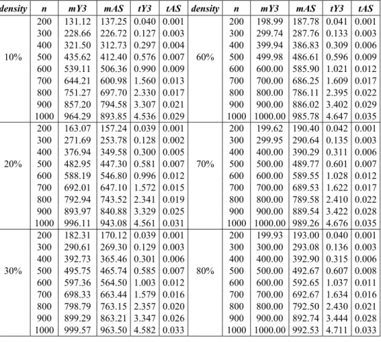
The second set of computational tests was designed to compare specifically Yuen3 and AS. A much larger quantity of instances, 2000, was used for each value of n ranging from 200 up to 1000 patterns and the results are presented in Table 2. The quantity of pieces and types were associated with the density of graphs Gmosp’s which varied from 10% up to 90%. AS produces much better results than Yuen3 in all classes. It becomes clear that AS is much faster than Yuen3, indeed, it is almost ten times faster for instances with high density and/or n large. It is worth of mentioning that for a given value of n AS has an almost equal time response in respect to the density. A possible explanation to understand this behavior can be the fact that a Gmosp has a large clique embedded in it and after sequencing it the induced graph becomes very sparse. The existence of a large clique detected by MDGh can also be a possible reason of why by imposing just two rotations to Erh sets Con and Rem have small cardinality. The suggested AS heuristic dominates Yuen3 in experimental running times and means errors. It possesses a smaller complexity order and also it has a very simple implementation.
Algorithm AS implemented in C++ can be obtained directly by request from the corresponding author.
Table 2 – Comparison of Yuen3 and AS, randomly generated patterns × pieces. Time is expressed in seconds.
density n mY3 mAS tY3 tAS density n mY3 mAS tY3 tAS
200 131.12 137.25 0.040 0.001 200 198.99 187.78 0.041 0.001 300 228.66 226.72 0.127 0.003 300 299.74 287.76 0.133 0.003 400 321.50 312.73 0.297 0.004 400 399.94 386.83 0.309 0.006
10% 500 435.62 412.40 0.576 0.007 60% 500 499.98 486.61 0.596 0.009
600 539.11 506.36 0.990 0.009 600 600.00 585.90 1.021 0.012 700 644.21 600.98 1.560 0.013 700 700.00 686.25 1.609 0.017 800 751.27 697.70 2.330 0.017 800 800.00 786.11 2.395 0.022 900 857.20 794.58 3.307 0.021 900 900.00 886.02 3.402 0.029 1000 964.29 893.85 4.536 0.029 1000 1000.00 985.78 4.647 0.035 200 163.07 157.24 0.039 0.001 200 199.62 190.40 0.042 0.001 300 271.69 253.78 0.128 0.002 300 299.95 290.64 0.135 0.003 400 376.94 349.58 0.300 0.005 400 400.00 390.29 0.311 0.006
20% 500 482.95 447.30 0.581 0.007 70% 500 500.00 489.77 0.601 0.007
600 588.19 546.80 0.996 0.012 600 600.00 589.55 1.028 0.012 700 692.01 647.10 1.572 0.015 700 700.00 689.53 1.622 0.017 800 792.94 743.52 2.341 0.019 800 800.00 789.58 2.410 0.022 900 893.97 840.88 3.329 0.025 900 900.00 889.54 3.422 0.028 1000 996.11 943.08 4.561 0.031 1000 1000.00 989.26 4.676 0.035 200 182.31 170.12 0.039 0.001 200 199.93 193.00 0.040 0.001 300 290.61 269.30 0.129 0.003 300 300.00 293.08 0.136 0.003 400 392.73 365.46 0.301 0.006 400 400.00 392.90 0.315 0.006
30% 500 495.75 465.74 0.585 0.007 80% 500 500.00 492.67 0.607 0.008
200 192.18 178.46 0.040 0.002 200 200.00 194.40 0.043 0.001 300 296.44 276.81 0.131 0.003 300 300.00 294.58 0.137 0.003 400 398.50 376.85 0.305 0.005 400 400.00 393.88 0.317 0.006 40% 500 498.79 474.51 0.588 0.008 90% 500 500.00 493.65 0.609 0.008 600 599.45 574.54 1.008 0.012 600 600.00 593.63 1.040 0.012 700 699.77 675.15 1.594 0.017 700 700.00 693.42 1.643 0.016 800 799.85 775.02 2.372 0.021 800 800.00 793.18 2.472 0.021 900 899.91 874.32 3.363 0.028 900 900.00 893.46 3.458 0.026 1000 999.97 973.74 4.604 0.034 1000 1000.00 993.14 4.725 0.033 200 196.91 184.01 0.041 0.001
300 299.04 283.37 0.132 0.003 400 399.64 382.88 0.306 0.006 50% 500 499.77 481.90 0.592 0.009 600 599.89 581.83 1.012 0.013 700 699.99 681.51 1.599 0.017 800 799.99 781.76 2.381 0.023 900 899.99 880.84 3.381 0.028 1000 1000.00 980.50 4.624 0.036
5. Conclusion
The Minimization of Open Stacks Problem appears directly in a large quantity of practical settings and it has a structure that makes it difficult to be solved exactly since it is also a NP-Hard problem. The very well known and simple heuristic for solving the problem – Yuen3 – produces good results in the practice, in the quantity of open stacks and in the running time, therefore it is difficult to find a better approach for the solving the problem. It was observed here that the problem when modeled as a search in a special graph – the MOSP Graph – possesses very large cliques. This feature permitted to be explored and a quadratic computational requirements time and space heuristic, AS was suggested. Extensive computational experiments were carried out and from them it is possible to infer that the suggested heuristic dominates Yuen (1991 and 1995) approach in the running time and mean error too. AS generated smaller quantities of open stacks than Yuen3, also it was always faster than the latter in the practice and in theory it improves the running time by a factor of n. Moreover, no heuristic can have a better theoretical order of convergence than AS since it allocates a time for solving the problem proportional to the input size.
Acknowledgments
We are greatly indebted to three anonymous reviewers whose thorough and detailed review helped pretty much us to greatly improve the manuscript. We would like to thank José Carlos Becceneri for sending us the code for the BYS04 heuristic and Horacio Hideki Yanasse for many helpful discussions too.
Dedication
References
(1) Angluin, D. & Valiant, L.G. (1979). Fast probabilistic algorithms for Hamiltonian circuits and matchings. Journal of Computer and System Sciences, 18, 155-193.
(2) Ashikaga, F.M. (2001). A frugal method for the minimization of open stacks problem. (in Portuguese) MSc. Thesis. Technological Institute of Aeronautics.
(3) Becceneri, J.C.; Yanasse, H.H. & Soma, N.Y. (2004). A method for solving the minimization of the maximum number of open stacks problem within a cutting process. Computers & Operations Research, 31, 2315-2332.
(4) Becceneri, J.C. (1999). The Minimization of Open Stacks Problem in industrial environments (in Portuguese). DSc. Thesis. Technological Institute of Aeronautics. (5) Bollobás, B. (1998). Modern Graph Theory. Springer, New York.
(6) Bollobás, B. (2001). Random Graphs. 2 edition, Cambridge University Press, Cambridge.
(7) Ferreira, A.G. & Song, S.W. (1992). Achieving optimality for gate matrix layout and PLA folding: a graph theoretic approach. Integration. The VLSI Journal, 14(2), 173-195. (8) Faggioli, E. & Bentivoglio, C.A. (1998). Heuristic and exact methods for the cutting
sequencing problem. European Journal of Operational Research, 110(3), 564-575.
(9) Fink, A. & Voss, S. (1999). Applications of modern heuristic search methods to pattern sequencing problems. Computer and Operations Research, 26(1). 17-34.
(10) Garey, M.R. & Johnson, D.S. (1979). Computers and Intractability: A Guide to the theory of NP-Completeness. Freeman, San Francisco.
(11) Halldórsson, M.M. & Radhakrishnan, J. (1994). Greed is good: approximating independent sets in sparse and bounded-degree graphs. Proc. STOC’94, 439-448. (12) Homer, S. & Peinado, M. (1996). Experiments with polynomial-time clique approximation
algorithms on very large graphs. In: Cliques. Coloring. and Satisfability: Second DIMACS Implementation Challenge [edited by D.S. Johnson and M.A. Trick], 26, 146-167. (13) Kučera, L. (1995). Expected complexity of graph partitioning problems. Discrete
Applied Mathematics, 57, 193-212.
(14) Linhares, A. & Yanasse, H.H. (2002). Connections between cutting-pattern sequencing. VLSI design and flexible machines. Computers and Operations Research, 29(12), 1759-1772.
(15) Pósa, L. (1976). Hamiltonian circuits in random graphs. Discrete Mathematics, 14, 359-364. (16) Yanasse, H.H. (1997a). On a pattern sequencing problem to minimize the maximum
number of open stacks. European Journal of Operational Research, 100, 456-463. (17) Yanasse, H.H. (1997b). A transformation for solving a pattern sequencing problem in
the wood cut industry. Pesquisa Operacional, 17(1),57-70.
(18) Yuen, B.J. (1991). Heuristics for sequencing cutting patterns. European Journal of Operational Research, 55, 183-190.